The Role of Data-Driven Instructional Models in the Development of Students’ Critical Thinking Skills in Core Literacy Education

Data publikacji: 17 mar 2025
Otrzymano: 17 paź 2024
Przyjęty: 28 sty 2025
DOI: https://doi.org/10.2478/amns-2025-0177
Słowa kluczowe
© 2025 Min Zhang, published by Sciendo
This work is licensed under the Creative Commons Attribution 4.0 International License.
Core literacy refers to a set of comprehensive abilities and literacies that individuals need to possess when facing complex problems and situations, and it is a basic ability and quality that can support individuals’ learning, work and life in different fields [1-2]. Core literacies include, but are not limited to, critical thinking, innovative thinking, cooperation, communication skills, information literacy, cultural literacy, emotional literacy, etc. These literacies not only help individuals solve problems and cope with challenges but also promote their personal growth and social development [3-5]. The appropriate teaching mode is the key to developing students’ core literacy. However, the current traditional teaching mode is not effective in developing students’ core literacy due to insufficient pre-course guidance and evaluation feedback from teachers, resulting in poor pre-course preview quality, in-class interaction level and higher-order thinking development [6-9]. In addition, the existing empirical studies related to the development of students’ core literacy are mostly result-oriented, lacking the support of data-driven system design and process dynamic data, and relying only on traditional teaching analytics tools. They cannot effectively monitor and reproduce the offline learning process of students, making it difficult to comprehensively and realistically measure the effectiveness of students’ learning [10-14]. Therefore, using learning analytics technology as an entry point to establish a data-driven teaching model oriented to core literacy can exercise students’ higher-order thinking skills and develop their core literacy [15-18]. For critical thinking, the data-driven teaching model promotes communication and interaction in the learning process through purposeful and organized judgment and dialogue, in which interpretation, analysis, evaluation and reasoning are generated, which provides an exercise field for developing critical thinking [19-21].
Based on the socio-spatial theory and the use and satisfaction theory, this study establishes a theoretical framework for the environment of the technical data-driven teaching model consisting of physical space, activity space and psychological space and analyzes its impact on the development of students’ critical thinking ability in core literacy education. The elements of physical space, activity space and psychological space in the teaching model were taken as explanatory variables, and the development of critical thinking ability as explanatory variables, respectively, and relevant questionnaires were designed and distributed in a school for data collection. Finally, descriptive statistical analysis, correlation analysis and regression analysis were performed on the data, respectively, to explore the practical significance of the data-driven teaching mode in promoting the development of students’ critical thinking ability.
Through the qualitative analysis of classroom observation data and student interview data, the key elements and their characteristics that support the development of higher-order thinking in high school language are analyzed from the real classroom context, and the theoretical model of the data-driven teaching mode to support the development of student’s critical thinking ability is constructed as shown in Fig. 1, combining with the previous understanding of the structure and function of the technology-enriched classroom environment.
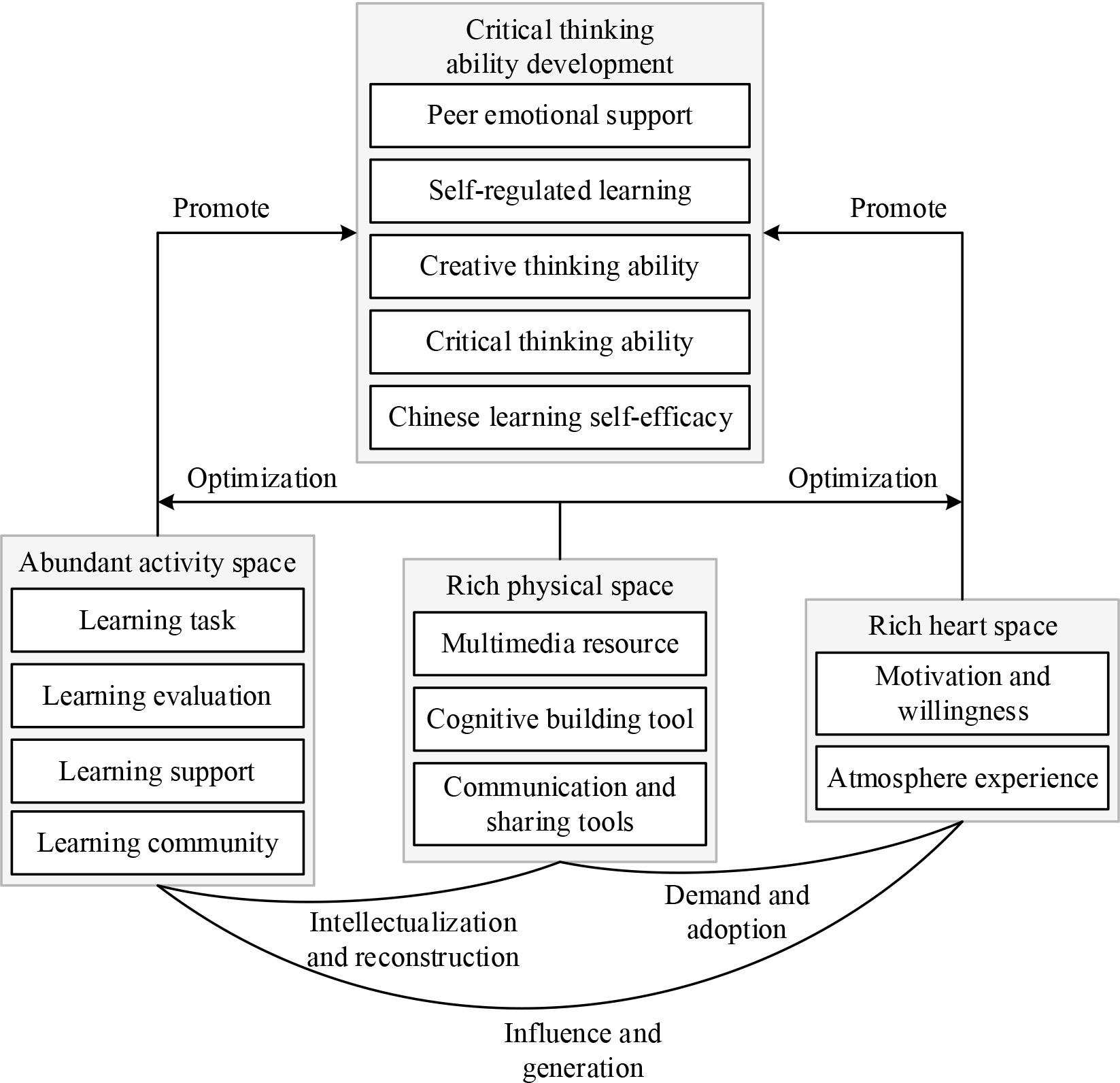
The theoretical model of students’ critical thinking ability development
The data-driven teaching model acts on the process of students’ critical thinking ability development with three dimensions of rich physical space, rich activity space and rich psychological space, and supports students’ critical thinking ability development. The theoretical model is explained below in terms of the interrelationships between three-dimensional spatial elements and their role in the development of higher-order thinking in high school language.
Hypothesis 1: The data-driven instructional model activity space element significantly promotes the development of student’s critical thinking skills in core literacy education.
Hypothesis 2: The physical space element of the data-driven instructional model significantly promotes the development of students’ critical thinking skills in core literacy education.
Hypothesis 3: The data-driven instructional model mental space element significantly promotes the development of student’s critical thinking skills in core literacy education.
Hypothesis 4: The data-driven instructional model shows a correlation with the development of students’ critical thinking skills.
In the pre-survey phase of this study, one prestigious high school, one high-quality high school, and one average high school were selected, and there was a large gap between the student population of the three high schools. The pre-survey included three grades of students, and one class was randomly selected for each grade. The “pre-survey” used on-site organization of the questionnaire mode. The two surveys issued 320 questionnaires and recovered 300 valid questionnaires, with a recovery rate of 93.8%.Among them, 135 were girls and 165 were boys.
Measurement Scale of Three Elements of Data-Driven Instruction
The connotation and characteristics of the key elements of the three-dimensional degree space of the data-driven teaching model have been portrayed in depth and detail in the previous section, according to which the observational indexes of the key elements of the three-dimensional degree space can be determined, as shown in Table 1. The internal consistency coefficient of the whole scale is 0.791.
Critical Thinking Skills Scale for Students
The California Critical Thinking Disposition Scale, or the Scale for short, has questionnaire questions derived from the personality traits proposed by the U.S. Delphi Item Group regarding critical thinkers. Corresponding attitudes are categorized into six levels, from strongly agree to strongly disagree, and subjects choose the option that best meets their attitudes among the six levels based on sentence descriptions. The scale has a total of questions, including seven dimensions: curiosity, openness, systematicity, truth-seeking, self-confidence, and maturity and the number of questions for each dimension is maintained at the question, with an overall reliability of 0.93 [22]. The Cologne Bach coefficients of the dimensions in the sample test results ranged from about 0.51 to 0.83, the Cologne Bach reliability coefficient of the whole scale was 0.88, and the internal consistency coefficient of the total scale in this study was 0.812.
| Observation dimension | Observation index |
|---|---|
| Physical space Active space | Multimedia resources |
| Cognitive construction tool | |
| Ac evaluation tool | |
| Observation dimension Physical space Active space | Learning task |
| Learning support | |
| Learning community | |
| Learning evaluation | |
| Observation dimension | Incentive will |
| Atmosphere experience |
Computational modeling
The multiple linear regression model is an extension of the univariate linear regression model, and its basic principles are similar to those of the univariate linear regression model, except that it is computationally more complex. A multiple linear regression model is an equation that describes how the dependent variable
Where:
When the original information establishes the multivariate regression model, in order to ensure that the regression model has excellent explanatory ability and predictive effect, the theoretical conditions that should be satisfied are:
Linearity: the relationship between the dependent variable and the independent variable is linear. That is to say, the independent variable has a significant effect on the dependent variable and has a close linear correlation. Independence, the random error term is independent across sample points with no autocorrelation. We have a random sample {( Mutual exclusivity: the independent variables should be mutually exclusive. That is, the degree of correlation between the independent variables should not be higher than the degree of correlation between the independent variables and the cause of the dependent variable. Completeness: the independent variables should be complete statistics, and their predictive values should be easy to determine. Normality, the random error term obeys a normal distribution with zero mean and variance. Variance uniformity: the random error term has equal variance at different sample points.
Estimation of biased regression coefficients:
One of the purposes of regression analysis is to develop regression equations that enable researchers to predict the value of the dependent variable based on the known independent variables. The estimation of the partial regression coefficients for a multiple regression model, like the same linear regression equation, is also done by solving the parameters by the least squares method, provided that the sum of squared errors (∑
The formula to derive
Solve this equation to find the value of
2) Tests of the model
Hypothesis testing of multiple regression model includes goodness-of-fit test, significance test of multiple regression equation as a whole with hypothesis test of partial regression coefficients.
A goodness-of-fit test is a test of the goodness of fit of a model to a sample of observations, which can be accomplished by constructing a statistic that expresses the degree of fit. The overall sum of squares
Goodness-of-fit test statistic decidable coefficient
The closer
The test of significance of the equation aims to make an inference about whether the linear relationship between the explanatory variables and the explanatory variables in the model holds significantly in the aggregate.
The original hypothesis
Obey the
Hypothesis test for biased regression coefficients: the
Since the model parameter
A statistic can be constructed as follows:
Given the significance level
The principle of correlation analysis is the process of analyzing the degree of correlation between two or more variables and expressing the results of the calculations through appropriate indicators. Variable selection generally consists of two parts: rules and query mechanisms. By rules, we mean the rules for evaluating the joint correlation between variables in a set of variables [24]. The main purpose of the query mechanism is to delete or add variables to the set of variables. Evaluation rules, also known as evaluation criteria, play a decisive role in variable selection. Both parts and feature construction are inseparable from correlation. Correlation is a general concept used to describe the degree of data closeness between variables and the amount of mutual information contained, including asymmetric causal and driving relationships. The basic idea of feature selection based on correlation analysis is to select effective variables with higher correlation with the prediction target, i.e., feature variables contributing to the performance of the prediction model, by analyzing the correlation strength relationship between variables.
Commonly used correlation coefficients:
Pearson’s correlation coefficient Define the aggregate of the two-dimensional variable
The means of variable
Equation (11) represents the mean of observed data for variable
Equations (13), (14), and (15) compute the covariance of the observations for variable
In matrix
Therefore the matrix
|
Where
In short, the absolute value of the Pearson coefficient is close to 1, which proves that the correlation between the two variables is stronger; on the contrary, the smaller the absolute value is, the weaker the correlation between the variables is, and the stronger the independence is. Meanwhile, it should be noted that the use of Pearson’s correlation coefficient needs to follow the following principles.
Pearson’s correlation coefficient is only applicable to linear correlation data analysis.
The calculation of the Pearson coefficient will have a greater impact when the observed data of the variables have extreme values.
Using the Pearson correlation coefficient, it is required that the two-dimensional overall (
2) Distance correlation coefficient
The formula for the distance correlation coefficient for the two variables
Where the covariance
The relevant term in the above equation is defined as:
The term of interest for the random variable
3) Information Entropy and Mutual Information
The concept of information entropy refers to the average amount of information in a message after eliminating redundancy, which is used to express the quantitative performance of the message. For a set of random variables
Where
For random variables
Among them:
The conditional entropy of
Mutual information in information theory denotes the interdependent inclusion of two variables
Where
Mutual information can also be represented by information entropy with the following formula:
The overall profile of the study population is shown in Table 2. Among them, 131 students belonging to quality schools (43.67%), 55% of the total number of females, 51.67% of the total number of students from urban areas, and 198 students from arts and sciences (66%), which is in line with the thinking characteristics of the development of critical thinking skills.
| Categories | Project | N | Percentage(%) |
|---|---|---|---|
| School | Elite school | 78 | 26 |
| Quality | 131 | 43.67 | |
| General | 91 | 30.33 | |
| Gender | Male | 135 | 45 |
| Female | 165 | 55 | |
| Grade | A high | 178 | 59.33 |
| High two | 122 | 40.67 | |
| Home | Countryside | 145 | 48.33 |
| City | 155 | 51.67 | |
| Disciplines | Liberal arts | 198 | 66 |
| Science | 102 | 34 |
The students’ CTDI-CV scores for each dimension and the percentage of critical thinking tendencies are shown in Table 3. The total score of students’ CTDI-CV is (293.14±30.6), which is positive critical thinking. The highest score in each dimension is curiosity, the lowest is self-confidence, and there are a few people who have positive and strong critical thinking in each dimension, in which the proportion of the number of people in the curiosity dimension (22.4%) is higher than the other dimensions.
| Project | Score(score, |
Each dimensional score distribution [n(%)] | |||
|---|---|---|---|---|---|
| Negative thinking(≤30 score) | Ambiguity(31~39 score) | Positive thinking(≥40 score) | Positive thinking(≥50 score) | ||
| Seek the truth | 43.25±6.09 | 32(18.2) | 48(31.2) | 78(49.3) | 11(6.2) |
| Liberation thought | 51.45±2.99 | 4(2.1) | 37(24.2) | 115(71.3) | 11(6.2) |
| Analytical ability | 51.24±1.13 | 4(2.1) | 48(31.2) | 97(62.1) | 16(9.6) |
| systematization | 48.26±2.56 | 11(6.3) | 67(42.7) | 78(49.3) | 11(6.2) |
| self-confidence | 43.52±5.72 | 22(12.2) | 79(48.51) | 61(38.3) | 9(5.8) |
| Thirst for knowledge | 52.23±5.28 | 6(2.3) | 46(38.5) | 82(51.3) | 35(21.4) |
| Cognitive maturity | 48.94±3.26 | 17(10.2) | 51(30.2) | 89(56.4) | 13(7.8) |
| Total score | 293.14±30.6 | 0(0.0) | 67(42.8) | 96(52.9) | 4(2.1) |
In order to examine whether there is a significant difference between the student’s critical thinking in terms of gender, an independent samples t-test was conducted on the students’ total critical thinking scores and their sub-dimension scores, and the results of the t-test are shown in Table 4. The table shows that although the mean of the total critical thinking scores of male students (266.19) is higher than that of female students (264.28), it does not reach a significant difference (P=0.598>0.05), so there is no significant difference between the total scores of the student’s critical thinking in terms of gender but there is a significant difference between the sub-dimensions of truth-seeking, self-confidence, and cognitive maturity, where the scores of male students are significantly higher than those of female students in the sub-dimensions of truth-seeking and self-confidence. Aspect boys scored significantly higher than girls, while in the cognitive maturity sub-dimension, girls scored significantly higher than boys.
| Male(N=35) | Fmale(N=165) | T value | Sig | |||
|---|---|---|---|---|---|---|
| M | SD | M | SD | |||
| Seek the truth | 37.81 | 6.836 | 36.13 | 4.751 | 2.084* | 0.041 |
| Liberation thought | 38.99 | 5.41 | 37.21 | 4.677 | 1.137 | 0.277 |
| Analytical ability | 38.93 | 6.011 | 39.18 | 5.777 | 0.522* | 0.639 |
| systematization | 35.75 | 4.863 | 36.02 | 4.712 | .344 | 0.769 |
| self-confidence | 38.91 | 6.398 | 36.11 | 5.493 | 2.566* | 0.011 |
| Thirst for knowledge | 39.85 | 5.675 | 41.42 | 6.576 | -1.349 | 0.16 |
| Cognitive maturity | 35.95 | 7.004 | 38.21 | 5.863 | -2.441* | 0.011 |
| Total score | 266.19 | 35.21 | 264.28 | 27.212 | -.431 | .598 |
*P≤0.05;**P≤0.01;***P≤0.001
Similarly, to examine whether there is a significant difference between students in terms of arts and sciences, we conducted an independent samples t-test. The differences in college students’ critical thinking in terms of majors are shown in Table 5, which shows that there is a significant difference between the students’ total scores of critical thinking in terms of majors (P=0.018<0.05). Also, there is a significant difference between the two subdimensions of truth-seeking and analytical ability, where the science students’ Critical Thinking is significantly higher than that of Arts students, and Science students’ scores in the two sub-dimensions of truth-seeking and emancipation are also significantly higher than that of Arts students.
| Science(N=102) | Liberal arts(N=198) | T value | Sig | |||
|---|---|---|---|---|---|---|
| M | SD | M | SD | |||
| Seek the truth | 37.12 | 6.845 | 35.84 | 5.648 | 2.145* | 0.041 |
| Liberation thought | 38.36 | 5.879 | 37.64 | 5.267 | 1.137 | 0.077 |
| Analytical ability | 39.69 | 6.711 | 38.44 | 6.171 | 2.084* | 0.039 |
| systematization | 36.08 | 5.715 | 35.84 | 5.071 | 1.123 | 0.169 |
| self-confidence | 36.56 | 7.313 | 37.84 | 5.857 | -.566 | 0.011 |
| Thirst for knowledge | 41.16 | 7.56 | 40.26 | 6.253 | 1.441 | 0.061 |
| Cognitive maturity | 38.12 | 7.878 | 37.27 | 6.185 | 1.349 | 0.076 |
| Total score | 267.09 | 25.421 | 263.13 | 32.534 | 1.898* | 0.018 |
*P≤0.05;**P≤0.01;***P≤0.001
Pearson correlation analysis was carried out to correlate the total score of students’ critical thinking ability with the total score and each factor of the data-driven teaching mode, and the results of the analysis are shown in Table 6. From the table, it can be seen that there is a significant correlation between the dimensions of students’ data-driven teaching mode and their critical thinking ability on the total score and some factors. On each factor, there is a significant correlation of 0.01 between the desire for knowledge, systematization ability and all factors in the data-driven teaching model. Truth-seeking was significantly correlated with physical and mental space. However, open-mindedness, analytical ability, and self-confidence in critical thinking were not correlated with the data-driven instructional model. There is a significant positive correlation between the total score and all factors of critical thinking skills of high school students, which confirms hypothesis 4.
| Project | Open mind | Thirst for knowledge | Cognitive maturity | Systematization | Look for the truth | Analytical ability | Self-confidence | Total score |
|---|---|---|---|---|---|---|---|---|
| Active space | 0.046 | 0.157*** | 0.033 | 0.122** | 0.068 | 0.042 | 0.052 | 0.113** |
| Physical space | 0.017 | 0.176*** | -0.008 | 0.173** | 0.092* | 0.081 | 0.078 | 0.132** |
| Psychological space | 0.041 | 0.174*** | 0.043 | 0.166** | 0.121** | 0.054 | 0.058 | 0.132** |
| Total score | 0.278 | 0.192** | 0.036 | 0.174** | 0.097* | 0.063 | 0.072 | 0.151** |
*P≤0.05;**P≤0.01;***P≤0.001
In carrying out the linear regression analysis, it is necessary to check whether there is multivariate covariance between the variables, which is judged by observing the values of eigenvalues, conditional indices, and checking the values of tolerance and variance inflation factor, and the diagnostic results are shown in Table 7. According to the data in Table 7, it can be learned that the value of the variance inflation factor of all dimensions is less than 10, the franchised value TOL is far away from 1, the eigenvalues are greater than 0.01, and the condition index is less than 30. Therefore, there is no multivariate covariance between the predictor variables, and it can be analyzed by using multiple regression.
| Dimension | Eigenvalue | Conditional index | Common linear statistics | |
|---|---|---|---|---|
| Authorized value | Coefficient of variance expansion | |||
| 1 | 0.012 | 19.231 | 0.523 | 1.231 |
| 2 | 0.031 | 17.452 | 0.532 | 1.892 |
| 3 | 0.022 | 19.224 | 0.611 | 1.593 |
The normal distribution plot is shown in Figure 2, in which the residual data from the regression analysis are evenly distributed on or near the diagonal and do not deviate very significantly, thus proving that the regression standardized residuals satisfy the normal distribution.
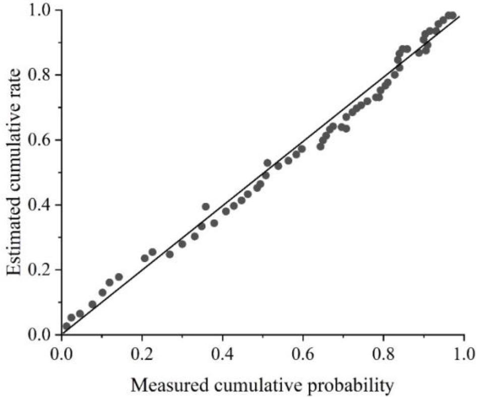
Normal distribution
The multiple regression analysis will be carried out by taking the activity space, physical space, and mental space elements as independent variables and the total score of students’ critical thinking skills in nuclear literacy education as dependent variables, and the results of the analysis are shown in Table 8. From the results of the regression analysis in the table, it can be seen that the fit of this linear regression is acceptable, R-squared = 0.296, and these four influences can together explain 29.6% of the variance in the total score of students’ development of critical thinking skills, and the R-squared is referred to as the coefficient of determination, which is used to measure the degree of fit between the regression straight line and the data. The F value is 53.052, p<0.001, which reaches the highly significant level, indicating that the model regression effect is better, and the B value of the three factors, activity space, physical space and psychological space factors, is greater than 0, and the significance is less than 0.05, which indicates that all three factors have a significant positive impact on the development of student’s critical thinking skills, which verifies the hypothesis 1, hypothesis 2, as well as the hypothesis 3 observation. Beta coefficients: The maximum value is in the activity space, followed by physical and mental spaces. Therefore, the magnitude of the influence of the three factors on the development of student’s critical thinking skills is activity space > physical space > psychological space. Entering into this regression model, the regression equation about the development of student’s critical thinking skills is students’ critical thinking skills = 1.088 + 0.182*activity space + 0.145*physical space + 0.121*mental space.
| Model | Non-standard error factor | Standard coefficientBeta | T | significance | |
|---|---|---|---|---|---|
| B | Standard error | ||||
| Constants | 1.088 | 0.142 | 8.314 | <0.001 | |
| Active space | 0.182 | 0.041 | 0.232 | 5.232 | <0.001 |
| Physical space | 0.145 | 0.038 | 0.193 | 5.088 | <0.001 |
| Psychological space | 0.121 | 0.036 | 0.095 | 3.145 | 0.032 |
| R2 | 0.296 | ||||
| F | 53.052 | ||||
| P | <0.001 | ||||
| Dependent variables: the total score of critical thinking in students | |||||
In this paper, 300 students from three universities were selected as subjects to study the relationship between the influence of a data-driven teaching model on the development of students’s critical thinking skills, and the results found that the students’ CTDI-CV total score was (293.14±30.6), positive critical thinking, and the highest score of all dimensions was inquisitiveness, and the lowest score was self-confidence, with the proportion of the number of people in the inquisitiveness dimension (22.4%) being higher than the other dimensions. Secondly, the level of critical thinking ability of male and female students is comparable, and there is no significant difference. However, science students possess better critical thinking abilities than those of arts students.
According to the results of multiple regression analysis, the F-value is 53.052, p<0.001, which reaches a highly significant level. The model demonstrates a superior regression effect. At the same time, the B-value of the activity space, physical space, and mental space factors is greater than 0, and the significance is less than 0.05. This indicates that all three factors have a significant positive impact on the development of the student’s critical thinking ability. This suggests that the data-driven model can significantly promote the development of the student’s critical thinking skills.