The Effect of Educational Resource Allocation on Teaching and Teaching Ability in Colleges and Universities Based on BP Neural Networks

Data publikacji: 17 mar 2025
Otrzymano: 04 lis 2024
Przyjęty: 08 lut 2025
DOI: https://doi.org/10.2478/amns-2025-0188
Słowa kluczowe
© 2025 Qian Wei, published by Sciendo
This work is licensed under the Creative Commons Attribution 4.0 International License.
In order to strengthen the management and utilization of high-quality educational resources and prioritize the development of a group of key universities and key disciplines to drive overall higher education, China launched the “211”, “985” construction program [1]. However, problems have emerged, such as stagnant development of universities, rigid identity, reduced competition, and low utilization of resources, which have affected the coordinated and sustainable development of higher education in China to a certain extent [2]. The current contradictory situation of limited resources and the expanding scale of higher education has made the allocation and utilization of higher education resources increasingly visible, and the development of higher education, education quality, and the efficiency of schooling have increasingly become hot topics of social concern [3-4]. China’s education development plans in previous years have centrally reflected the importance attached to the cause of higher education at the national level.
The finiteness or scarcity of higher education resources leads to the allocation of higher education resources and also raises the issue of fairness and efficiency in the allocation of higher education resources [5]. Higher education is the engine and gas pedal for realizing knowledge innovation and transforming scientific and technological achievements into productive forces, undertaking the important task of training and creating socialist builders and reliable successors, and carrying the sacred mission of realizing the great rejuvenation of the Chinese nation, “Chinese Dream”. At present, China’s higher education resource allocation mainly exists in the total amount of resources is insufficient, the distribution is uneven, the contradiction between demand and supply is prominent, and the role of the market mechanism as the main body of educational resource allocation is not enough to play the role of other problems [6-8]. Along with the deepening of the economic system reform, the reform in the field of education needs to be deepened, and the value and potential of resource allocation need to be further explored [9].
The resource structure imbalance factors in various higher education resource allocation systems will ultimately affect the overall efficiency of higher education [10]. Quantitative analysis using the dynamic development model can grasp the correctness of the current and future measures of higher education resource inputs, adjust and regulate the macro-financial policy of higher education in a timely manner so as to truly reflect the overall operational goals of higher education (the unity of efficiency and equity) [11-12].
Literature [13] points out that the allocation of educational resources is related to the location of the school but also the grade of the school. The higher the grade of the school, the more educational resources are allocated, and vice versa, the less. Literature [14] standardized educational resources into three main areas, including teacher quality, school physical environment and school teaching environment. Literature [15] suggests that for earmarked grants to influence local resource allocation as intended by the central government, strong enforcement mechanisms are necessary, but this may come at the cost of reducing local flexibility. Literature [16] mentions that government expenditures can be used for a variety of socio-economic objectives, including resource allocation for education, consumption of public goods and services, and social protection. Literature [17] expresses that the regional pattern and structure of HEIs have a significant positive effect on the overall maturity of the carrying capacity of higher education resources. Literature [18] expresses that developing the employability of higher education students is an important issue in higher education, and if colleges and universities with sufficient educational resources, the quality of education will be subsequently improved, and the results of teaching and learning will be more obvious, and the employability of students will be strong. Literature [19] strengthens the allocation of resources to higher education institutions through the creation and dissemination of knowledge, research, education and outreach activities so that higher education institutions are better able to realize the path of sustainable development. Literature [20] emphasizes that the development philosophy of higher education directly affects the direction of development of higher education because the philosophy usually reflects people’s understanding of the laws of higher education, and the current educational philosophy constrains the scale, quality, structure, and effectiveness of higher education to a certain extent.
In this paper, we first optimize the BP neural network using the PSO algorithm to establish a mapping relationship between the dimension space of PSO particles and the neural network connection weights and thresholds. Then, the educational resource allocation model is constructed based on the optimized BP neural network. The input layer is processed by determining the number of network layers to allocate educational resources based on the sample data input.Determine the number of nodes in the hidden layer and the number of neurons in the output layer, and select the transfer function, training algorithm, and related training parameters. Input the input samples into the neural network, calculate the error between the actual output value of the network and the target sample, and use the selected training algorithm to repeatedly modify the connection weights of the network until the error reaches convergence within the target error accuracy. Finally, the model is applied in practice to analyze the balance and comprehensive efficiency before and after the allocation of educational resources.
The flow of the PSO algorithm is shown in Fig. 1.
Initialization of particles. In a cluster of particles of size
Calculate the adaptation value and objective function for each particle.
For each particle, compare its adaptation value with its experienced best position Pbest, and if the adaptation value is better than Pbest, it is taken as the current best position Pbest.
For each particle, compare it with the best position Gbest experienced by the group, and if the adaptation value is better than Gbest, then it will be used as the best position of the group and reset the index number of Gbest.
Adjust the current position and velocity of the particles according to the following equation:
Check the termination conditions. Usually the maximum number of iterations
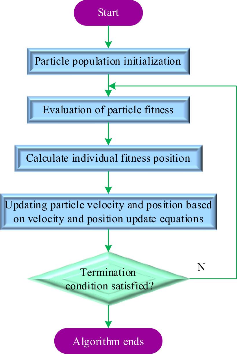
PSO algorithm chart flow
The particle swarm algorithm is a simple, effective stochastic search algorithm, which is based on the speed displacement search model, is simple to operate, has low computational complexity, and its use in the training of BP networks can avoid the defects of the local optimum of the BP learning algorithm. The training of the BP network can be divided into two types. One is to narrowly train the connection weights of the fully connected structure under the BP network. One is to train the BP network in a broad sense, such as optimizing the connection structure of the BP network and removing redundant connections while training the weights. Redundant connections may affect the classification performance of the BP network, so removing redundant connections eliminates this undesirable effect.
The PSO algorithm optimizes the neural network by training the weights and thresholds of the network instead of using the gradient descent method.The key is to establish the mapping relationship between the dimension space of PSO particles and the connection weights and thresholds of the neural network.The neural network learning process mainly involves updating weights and thresholds, while the PSO search process mainly involves changing speed and position in different dimensions. Thus, the weights and thresholds in the BP algorithm should correspond to the positions of the particles. The fitness function of the particle is the minimum mean square error MSE:
The specific steps of PSO training neural network weights are as follows:
Step 1: Determine the neural network structure, including the number of neurons in the input layer, hidden layer, and output layer. Step 2: Initialize the particle swarm. The dimensions of the particle position and velocity vectors, the values of which are the ownership value and the threshold value. Size of particle swarm Initialize the learning factors Initialize the particle swarm and the velocity of each particle. Initialize a two-dimensional matrix Initialize the individual extreme value and the global optimum value of each particle and record the corresponding weights and thresholds. Step 3: Determine the fitness function. The minimum mean square error MSE of the neural network is used as the evaluation index (fitness) of the particle search performance, which is used to guide the search of the population. Step 4: Perform a forward propagation calculation for each particle using all the training samples to generate the training error generated by the particle under the training samples. Step 5: Update the individual extremes and global optimum according to the fitness of each particle. For each body particle, if its current fitness is less than the individual extreme value before iteration, then individual extreme value update Step 6: Update the weighting coefficients Step 7: Update the velocity and position of each particle. Step 8: Judgment of algorithm stopping condition. Evaluate the fitness of the new particle population generated by the iteration and determine whether the algorithm reaches the maximum number of iterations or reaches the specified error criterion. If the conditions are met, then go to step 9; otherwise, the number of iterations is increased by 1 and then return to step 4 to continue the iteration. Step 9 generates the optimal solution. When the algorithm stops iterating, the global extreme value corresponding to the neural network weights and connection structure is the optimal solution to the training problem.
From the above description, it can be seen that the value of each element of the particle vector consists of the weights and thresholds in the BP network. The fitness function of the particle is also obtained based on the mean square error of the BP algorithm, which integrates the PSO algorithm and the BP algorithm.Figure 2 depicts the flow of the optimized BP algorithm.
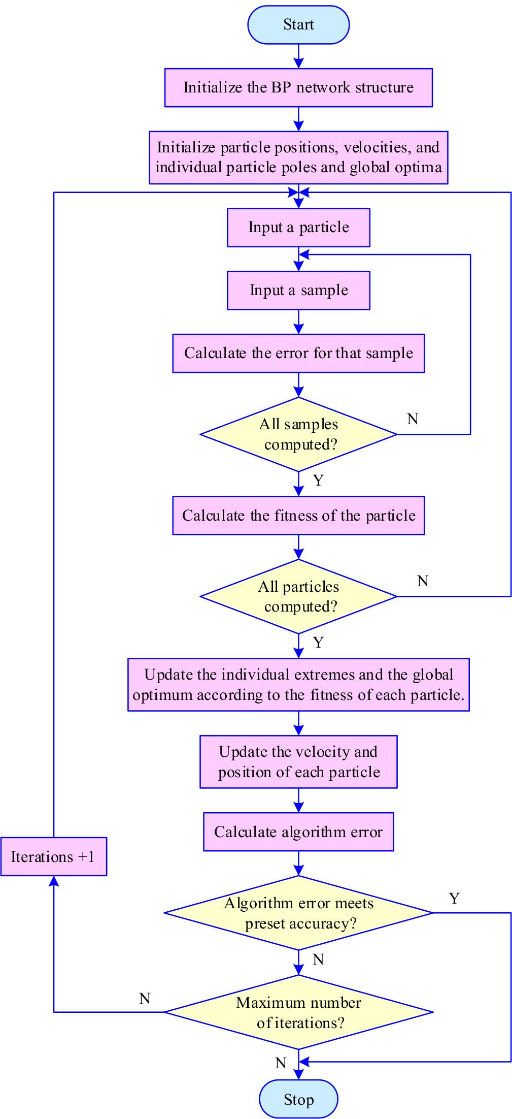
BP neural networks which trained by PSO algorithm chart flow
Analysis of input layer variables
BP neural network is the process of reducing the error between the learning sample data and the target sample through continuous and repeated learning, and finally training it into a system model. Therefore, to construct the BP neural network model of educational resource allocation, what needs to be determined is the data of the input layer variables, i.e., the learning samples. The selection of learning samples generally follows two principles: first, the selected samples have a greater impact on the output and are typically representative. The second issue is that the correlation of the learning sample is low.
Processing of input data
In MATLAB, the learning samples we collected are input into the model in the form of a matrix due to the different significance of the physical quantities of the selected indicators in the evaluation system we have identified. The order of magnitude of the vectors is somewhat different, and if the direct application of the original data is likely to cause the formation of large fluctuations in the measured values, affecting the training of the neural network, the data is usually normalized first. All the data are transformed into [0.1] or between [-1.1]. The normalization of the data, to avoid the formation of network learning error, is large because of the large differences in the input data, which is conducive to improving the training speed of the network and accelerating the convergence.
There are usually two methods of data normalization: the first max-min method. The formula is as follows:
The second method of mean variance. The formula is as follows:
In educational resource allocation, we apply the first method to normalize the collected raw data.
The hidden layer is the intermediate layer connecting the input layer and the output layer, which plays a decisive role in the performance of this neural network. Therefore, determining the number of nodes in the hidden layer is very important.
At present, there is no scientific and general theoretical method for determining the number of nodes in the hidden layer, and it is often derived from empirical formulas and practical experiments. The following are several empirical formulas summarized through some literature:
Golden section based optimization algorithm for the number of nodes in the hidden layer:
Regarding educational resource allocation through BP neural networks, qualitative input will be converted into quantitative output, and the final result will be evaluated comprehensively to provide a qualitative evaluation of the level of educational resource allocation.Therefore, the output layer is the result of allocation of educational resources. Here, in order to be able to analyze the configuration results in a more specific way, we classify the resulting configuration results into levels, and the evaluation level classification is shown in Table 1. The number of neurons in the output layer is 4.
Evaluate the hierarchical class
| Level | v | g | a | b |
| Content | Very good | Good | Acceptable level | Differ from |
| Desired Output | [1,0,0,0] | [0,1,0,0] | [0,0,1,0] | [0,0,0,1] |
The mathematical model of an artificial neuron consists of three main functions: weighting, summation, and transmission. Different transfer functions give neurons different information processing properties, resulting in different types of artificial neural networks.
Transfer functions
Linear function
The linear function is the simplest transfer function and is also known as the linear continuous model. The output of this function is proportional to the combined effect that the input has. The mathematical expression is:
Threshold function
The threshold function is a discrete output function. The output value is only 0 or 1. The mathematical expression is:
Nonlinear functions
Nonlinear functions are an extremely important type of function in transfer functions, i.e., type S functions. The most common are the
Sigmoid function and hyperbolic tangent function.
The formula for the Sigmoid function is:
The hyperbolic tangent function is given by:
The Sigmoid function has an output value range of [0,1], while the hyperbolic tangent function has an output value range of [–1,1]. Therefore, these two functions are often used when the output requirement is in this range.
Conceptual function
The conceptual transfer function takes the probability that the output state of a random function is 0 or 1, and is usually applied when the relationship between the input and output of a model neuron is uncertain. The mathematical expression is:
In the educational resource allocation model in this paper, we are utilizing the Sigmoid function as the transfer function.
According to the above understanding of BP neural network, establish a BP neural network. The input layer is the initial stage, and the input variable is the index for educational resource allocation. The middle layer is the hidden layer. By adjusting the weights of neurons, the actual samples are close to the target samples for educational resource allocation. The last layer is the output layer. The output data and network output can be adjusted accordingly to obtain the configuration results.
The specific training flow chart of educational resource allocation is shown in Figure 3. The specific steps are as follows: (1) Determine the number of network layers for educational resource allocation. (2) Process the sample data input from the input layer. (3) Determine the number of nodes in the hidden layer and the number of neurons in the output layer, and select the transfer function, training algorithm and related training parameters. (4) Input the input samples into the neural network, calculate the error between the actual output value of the network and the target sample, and use the selected training algorithm to repeatedly modify the connection weights of the network until the error reaches convergence within the target error accuracy. (5) Input test samples and judge the test results. If the network generalization ability is better, it means that the network design of educational resource allocation is completed.
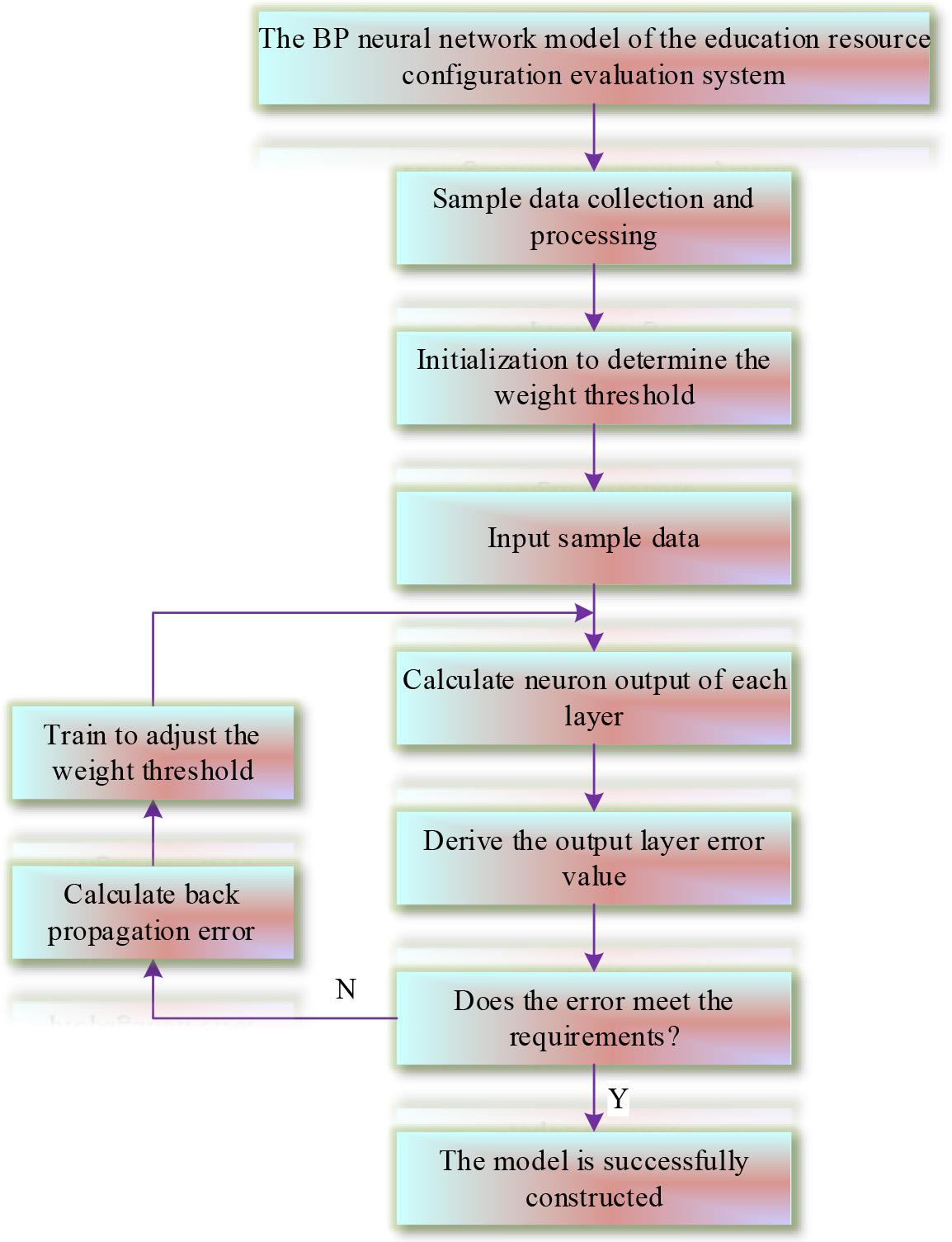
Education resource configuration training flow chart
Taking 15 colleges and universities in the university district of province H as the research object, an optimized BP neural network-based resource allocation model is used to allocate resources to each college and university.
This chapter designs the following solution process for the optimization of educational resource allocation in the university district:
Count the raw data of the compulsory education stage in the university district in each index and preprocess the raw data. Apply the optimized BP neural network resource allocation model to analyze the optimization results, the balance before and after resource allocation, and the comprehensive efficiency before and after resource allocation. The teaching and teaching ability of universities after resource allocation are analyzed against each other.
The results of the optimization of the allocation of educational resources in the university district are shown in Table 2. Taking the 1st university as an example, the total area of teaching and auxiliary rooms at the university is 22,368 square meters after allocation optimization. The total number of books after allocation optimization is 342978. The total number of computers after allocation optimization is 1142. The optimized value of teaching equipment is 1115 yuan. The optimal allocation of the total area of the sports field is 1,876 square meters.
Education resource allocation optimization results
| A | B | C | D | E | |
| 1 | 22368 | 342978 | 1142 | 1115 | 1876 |
| 2 | 25139 | 326393 | 1027 | 1209 | 1902 |
| 3 | 33283 | 443335 | 1606 | 1741 | 2183 |
| 4 | 33047 | 401181 | 2162 | 1444 | 3438 |
| 5 | 33208 | 328174 | 1181 | 726 | 2795 |
| 6 | 27016 | 345810 | 1257 | 2164 | 1888 |
| 7 | 20200 | 200206 | 795 | 1380 | 1272 |
| 8 | 29730 | 319980 | 1185 | 1279 | 1964 |
| 9 | 17174 | 397496 | 1222 | 1450 | 954 |
| 10 | 23559 | 274153 | 1143 | 1549 | 2558 |
| 11 | 25792 | 269829 | 1391 | 1278 | 1496 |
| 12 | 31220 | 282596 | 1419 | 2744 | 1612 |
| 13 | 14444 | 169864 | 1265 | 909 | 1121 |
| 14 | 80203 | 796287 | 4204 | 8546 | 6377 |
| 15 | 93035 | 643165 | 4286 | 7520 | 7336 |
The equalization of educational resource allocation before and after the university district is shown in Figure 4. The coefficient of variation of educational resource allocation of the 3rd college and the 12th college in the university district is 0.76 before the experiment of educational resource allocation, and after the experiment of educational resource allocation, the coefficient of variation of educational resource allocation is 0.49 and 0.58, respectively. After the allocation of educational resources, the variability of educational resource allocation within the university district becomes lower, which indicates that there is a tendency to equalize the development of individual colleges and universities.
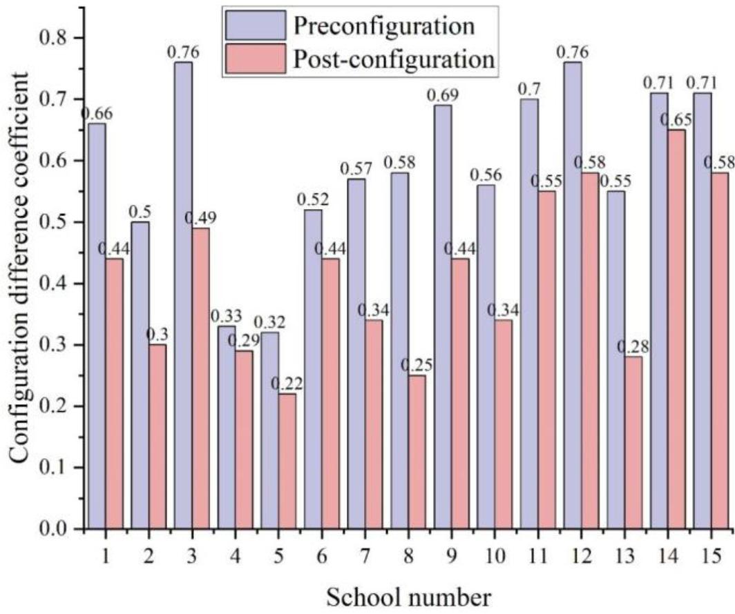
The balance of education resource allocation was compared
The combined efficiency of each university before and after the allocation of educational resources is shown in Figure 5. The horizontal coordinates of the figure represent each university, with the name of the university replaced by a number, and the vertical coordinates of the figure represent the comprehensive efficiency of the corresponding resources of each university obtained by calculation. The green line represents the comprehensive efficiency of educational resource allocation before the experiment, and the purple line represents the comprehensive efficiency of educational resource allocation after the experiment. It can be seen that before the experiment, the overall efficiency of resource allocation among colleges and universities was relatively low, except for individual colleges and universities. After the experiment, the comprehensive efficiency of the colleges all increased, the first college increased from 6.02151 to 10.75835. The second increased from 6.19212 to 10.84008. The highest increase in comprehensive efficiency was in the 8th college, which increased by 6.46782. the comprehensive efficiency of the educational resources allocation after the comprehensive efficiency converges to the equilibrium state.12 It can be shown that the model improved the efficiency of the university’s district resource efficiency and reduced the differences between colleges.
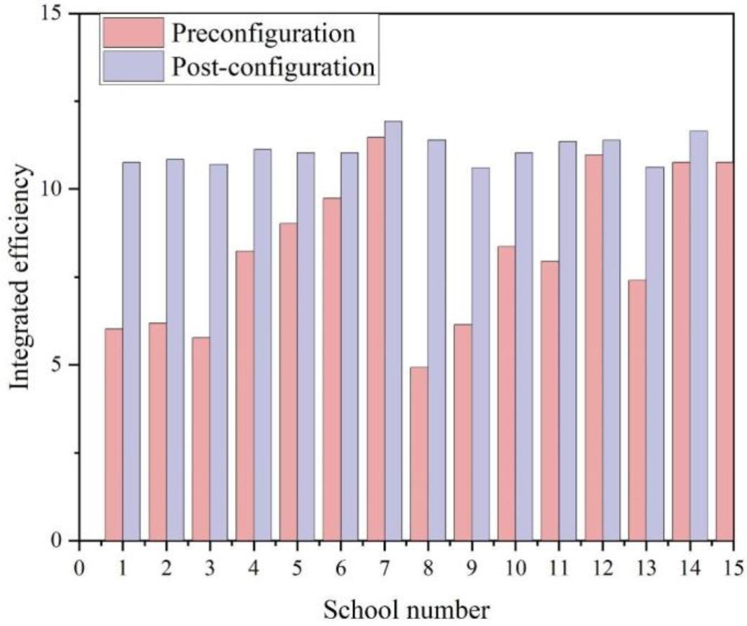
The comprehensive efficiency contrast of universities
The three aspects are analyzed through the optimization results of educational resource allocation, the balance comparison before and after educational resource allocation and the comprehensive efficiency comparison before and after educational resource allocation. It can be seen that this model has the effect of making each index reach the standard, reducing the differences between universities, and improving efficiency. The experiment shows that it is necessary to optimize the allocation of the existing resources in the university district of province H. It also verifies the correctness and usability of the model and the importance of the optimization of the allocation of educational resources, and provides theoretically based decision-making guidelines for the allocation of educational resources in the university district.
In order to verify the impact of the optimization of educational resource allocation on the teaching and learning ability of colleges and universities, this paper explores the changes in student achievement through teaching experiments. The experimental research object will be selected from any university in the university district of province H. The independent sample test of students’ post-test scores before and after the allocation of educational resources is shown in Table 3. Through the independent samples t-test, the significance level of the variance chi-square test is 0.000<0.05, which can indicate that there is a significant difference between the student’s performance before and after the allocation of educational resources, and it can be seen that the student’s performance after the optimization of the allocation of educational resources is significantly improved relative to the optimization of the pre-existing students’ performance.
Independent sample inspection
| Levin variance equivalence test | Average equivalent t test | 95% Confidence Interval of the Difference | |||||||
| F | Sig. | t | Freedom | Sig.(2-tailed) | Mean difference | Standard error difference | Lower | Upper | |
| Assumed equal variance | 1.325 | 0.257 | 4.341 | 75 | 0.000 | 8.4526 | 1.8365 | 4.235 | 12.56 |
| Unassuming equal variance | - | - | 4.332 | 73.245 | 0.000 | 8.4526 | 1.8324 | 4.136 | 12.59 |
This paper takes 15 colleges and universities in the university district of province H as the research object and analyzes the constructed educational resource allocation model.
After the allocation of educational resources, the variability of educational resource allocation of all 15 colleges and universities within the university district becomes lower. The highest comprehensive efficiency after educational resource allocation is improved by 6.46782, and the comprehensive efficiency all tends to the equilibrium state12. The model improves the efficiency of resources in this large school district and reduces variability among colleges and universities.
The significance level of the independent sample test of students’ post-test scores before and after educational resource allocation is 0.000<0.05. It shows that the optimization of educational resource allocation can improve the teaching and instructional capacity of universities.