Multivariate model optimisation during the implementation of flexible interconnection projects for MV distribution networks

Pubblicato online: 17 mar 2025
Ricevuto: 05 nov 2024
Accettato: 17 feb 2025
DOI: https://doi.org/10.2478/amns-2025-0186
Parole chiave
© 2025 Xing Su et al., published by Sciendo
This work is licensed under the Creative Commons Attribution 4.0 International License.
As a carrier of distributed renewable energy consumption and grid-connected services, the distribution network has been transformed from a power network purely used for power distribution to a hub platform with the functions of power transmission, distribution, storage and trading, including the higher-level power grid, local distributed renewable power generation, multiple loads, energy storage and other elements [1-4]. As the role of the hub platform becomes more and more prominent, the pressure of distribution network operation is increasing, and the construction of a “flexible and controllable, green and safe” new distribution network has become a major issue for the current and even the future period [5-7]. In order to cope with the new challenges faced by distribution grids, such as the consumption of distributed renewable energy power generation, the substitution of terminal electric energy such as coal to electricity, and the sharp increase of electric loads caused by electric vehicles etc., there are a series of possible forms of future distribution grids, including low-voltage direct current (DC) energy storage microgrids, energy local area networks (LANs), point-to-point structures, flexible distribution grids, and honeycomb distribution grids, etc. [8-11]. Among these possible forms, flexibility is one of the important characteristics of future distribution grids, which is specifically manifested in the distribution system’s ability to be resilient when there are uncertainties within or outside the distribution grid [12-13].
In recent years, the rapid development of distributed generation and other reasons have caused a large increase in the problems faced by medium-voltage distribution networks, such as two-way power flow and line overload. The flexible interconnection technology of the distribution network combines the flexible control technology of power electronics with the optimal design of the distribution network grid [14-17], which can provide fast and accurate active and reactive power control, power loss support and power quality management functions between distribution network lines and stations, and provides an effective technical means for tapping the power supply potential of the distribution network and improving the reliability of power supply, and is an important technical route to solve the high proportion of distributed power generation consumption in the distribution network [18-21].
In this study, flexible interconnection engineering is firstly analyzed in depth, the interconnection engineering technology and interconnection devices are introduced in detail, and the classical functional model of flexible interconnection system is analyzed. On this basis, this paper implements a multivariate model optimization of the distribution network based on B2B VSC, MMC-type B2B VSC and D-UPFC technologies. Based on the flexible interconnection project, the anti-islanding strategy, flexible interconnection optimization scheduling, and trend control optimization model were constructed. It is also verified through simulation experiments to evaluate the effects of three classical strategies, namely current inner-loop control, voltage outer-loop control, and power outer-loop control. Finally, the effects of this paper’s flexible interconnection engineering in practical applications are studied based on real data from the power grid in K province.
Most of the distribution network adopts “closed-loop design, open-loop operation”, using contact switches to form a hand-in-hand or mesh distribution network in each sub-district to realize sectional control and post-accident load transfer. However, as the electrification of urban and rural areas continues to increase, the load on the distribution network also increases, and the daily peak-valley difference gradually expands. At the same time, the penetration rate of distributed power supply and charging pile is gradually increasing, and the problems of new energy consumption, load gap, and power quality are becoming more and more prominent. The traditional distribution network adopts the “closed-loop design, open-loop operation” mode, which cannot realize the trend control, and the low voltage at the end of the line and other problems are increasingly visible.
The flexible interconnection device (FID) based on a power electronic device (PED) can realize the closed-loop interconnection between different AC divisions. By controlling the current of the DC link, the power equalization between different AC sub-divisions can be accomplished without considering the frequency synchronization problem. Compared to distribution network sectionalized switches and contact switches, FID technology makes fault isolation easier, which greatly improves the flexibility and safety of distribution network control. When FID technology is used for feeder interconnection of MV distribution network, asynchronous loop operation between multiple AC distribution feeders can be accomplished without increasing the short-circuit capacity, which can play the roles of trend transferring, load ratio balancing, network loss reduction, fault isolation and power supply restoration, etc., and realize the multi-terminal loop operation of feeders and optimal allocation of adjustable resources.
The flexible interconnection system of power supply sub-districts is shown in Fig. 1, in which two neighboring power supply sub-districts realize real-time interconnection of two regional power supply networks through flexible interconnection devices. The flexible interconnection device consists of two bi-directional AC/DC converters and realizes the flexible control of power supply inter-area currents by means of intelligent fusion terminals. Combined with the distribution master system, it realizes the optimized coordination of source, network, load and storage of the interconnection system, which improves the reliability and flexibility of the power supply of the distribution network system. Similarly, this technology can be applied to low-voltage flexible DC interconnection between two stations to solve operational problems such as difficulty in capacity increase of urban power grid, uneven load ratio of neighboring stations and low terminal voltage.
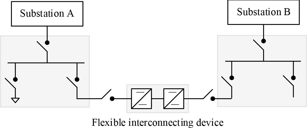
The power supply zoning soft interconnection system
The flexible interconnection device is the core equipment of the flexible DC interconnection system for power supply zones, and compared with the conventional contact switch, it has the functions of active scheduling, reactive power support, islanding power supply, load transfer and so on. Flexible interconnection devices have two or more access ports to meet the flexible interconnection of lines of different wiring modes, while DC access ports can be set up to meet the needs of accessing distributed power sources, DC loads and energy storage devices.
According to different distribution grid interconnection patterns, combined with the differences in AC system operation characteristics, as well as the concerns of each application scenario for specific needs such as high power supply reliability, load rate balance control, distributed power consumption and fluctuating power suppression, the functional modes of the distribution flexible interconnection system also differ.
For different application scenarios, the typical functional modes of various flexible interconnection systems can be summarized into the following categories:
Feeder load rate equalization According to the requirements of monitoring and controlling the transmission power of the FIDVSC connected to the AC feeder, thus realizing the equalization of the load rate of each feeder. The average feeder load factor where For the purpose of average load factor, the FID-VSC connected to AC feeder Multi-area system trend supply transfer When a certain feeder of the flexible interconnection system is out of operation, it is necessary to adjust the operation mode of other AC distribution stations and modify the FID-VSC power reference value connected to each feeder to complete the power transfer, realizing rapid load transfer and uninterrupted power supply for sensitive loads. When the AC feeder Where For AC feeder Where Fluctuating power supply power equalization The fluctuating power value of the distributed power supply is derived by detecting the fluctuating power connected feeder power value and subtracting the daily load value of that feeder. The low-frequency component value of this fluctuating power is assigned to each feeder according to the capacity of each feeder as the weight value and is used as the reference value of the FID-VSC operating power, so as to reduce the impact of the distributed power supply’s centralized access to a certain feeder on the normal operation of the interconnected distribution system:
Where In order to realize the power equalization of the fluctuating power supply, the active command value Where High quality power supply For AC loads and new DC loads with high demand for power supply reliability and quality, the AC power supply from the DC inverter of FID-VSC and the direct power supply after the DC transformer is adopted, with no harmonic and voltage dips. Dynamic reactive power compensation According to the need, change the reactive power value of FID-VSC connected to the feeder to provide a dynamic reactive power compensation function to the substation. In addition, the feeder voltage level needs to be dynamically adjusted according to the load side reactive power changes. According to the detected feeder voltage level, the reactive command value of FIDVSC is adjusted through feedback control to maintain the AC feeder voltage. For the FID-VSC equipment connected to AC feeder Where
The islanding effect in distribution networks can seriously threaten the life safety of distribution network operations and inspection personnel. Most of the existing anti-islanding strategies need to be specially configured for disturbed loads according to different sensitivity requirements, reliability requirements, and capacities, which will not only result in a waste of resources but also consume manpower.
In order to solve the above problems, this section proposes an anti-islanding strategy with self-adaptive capability for distribution networks based on back-to-back voltage-source converter (B2B-VSC) based on flexible interconnection engineering. The structure of the B2B VSC is shown in Fig. 2, and
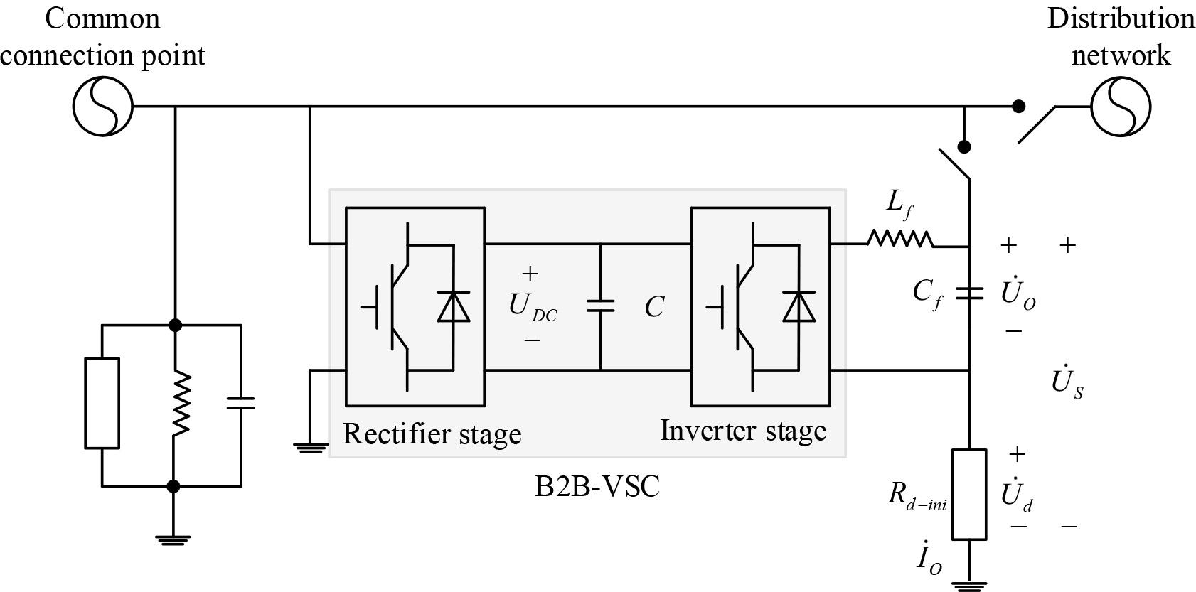
Basic structure of adaptive low-voltage anti-islanding strategy
The B2B-VSC can output a specified voltage phase
If the undervoltage protection alone is used to realize the low-voltage anti-islanding strategy, the perturbation load unit needs to exhibit a purely resistive characteristic with a phase relationship that indicates the equivalent load value of the perturbation load unit
In the conventional low-voltage anti-islanding strategy, if undervoltage protection is used, the perturbed load configuration is modeled as:
Where,
The equivalent load value of the perturbation load unit if the B2B-VSC based adaptive anti-islanding strategy is used:
It should be noted that since the active power consumed/emitted at the output of the B2B-VSC is equal to the power emitted/consumed at the input, the active power of the B2B-VSC is constant at 0, and the active power of the perturbed load cell includes only the power dissipation of
According to Eq. It can be seen that the resistance value of
If, in order to improve reliability, Undervoltage protection and over/underfrequency protection are used to realize low-voltage anti-islanding, the disturbing load unit needs to present resistive-inductive (dual protection of undervoltage and overfrequency) or resistive-capacitive characteristics (dual protection of undervoltage and underfrequency). It should be noted that, due to the external load quality factor
In the traditional low-voltage anti-islanding strategy, if Undervoltage and over-frequency double protection are used, the resistance configuration model of the disturbed load is the same as equation (1), and the inductive resistance configuration model of the disturbed load is
Where
In the traditional low-voltage anti-islanding strategy, if undervoltage and underfrequency double protection are used, the perturbed load resistance configuration model is the same as above, and the perturbed load capacitive reactance configuration model is:
Where,
The equivalent load impedance of the perturbation load unit if the B2B-VSC based adaptive anti-islanding strategy is used:
According to Eq. 1, the value of
Therefore, with the B2B-VSC-based adaptive anti-islanding strategy, the disturbed loads no longer need to be reconfigured when any one of the sensitivity requirements, reliability requirements, or DG capacity changes.
Since the traditional distribution network control method relying on “hard” switches cannot meet the demand for flexible and active trend regulation, this study introduces the intelligent soft on/off switch (SOP) to adapt to the needs of the smart grid construction, and the MMC B2B has the ability of flexible trend regulation and control, which can realize real-time, fast and smooth power control, and guarantee inter-area trend mutual aid. It can achieve real-time, fast, and smooth power control, guarantee mutual aid in inter-area trends, and greatly improve the reliability and flexibility of the distribution network.
The MMC B2B is based on a new type of power electronic device, which adjusts the power output value of the converter in real time by controlling the command value, so as to change the system’s current distribution. In this paper, a flexible interconnected substation system architecture using MMC B2B to replace traditional circuit breakers and sectionalized switches is proposed for low-voltage distribution networks, and the flexible interconnected substation system architecture is shown in Fig. 3. B2B-MMC consists of MMMC2, with Bus interconnection. It realizes inter-regional energy intercommunication and reactive power compensation functions and provides mutual support for the busbar voltage. Main transformer load balancing. Reduce the risk of equipment overload and improve power supply reliability. Non-stop power transfer. Realize rapid isolation when the main transformer fails and rapid recovery of non-fault areas, and enhance system stability. System trend optimization. The flexible interconnection state can enhance the transmission capacity of the distribution network as well as enrich the line transmission path, which is conducive to realizing the optimal distribution control of the system trend.

Flexible interconnection substation system architecture
When the flexibly interconnected substation with B2B-MMC is put into operation, QF and QC are in the disconnected state.
In the flexible power distribution system based on B2B-MMC, the communication state between converter stations is categorized into communication control and no-communication control according to different operation scenarios. Master-slave control is used in the communication control state, and voltage sag control is used in the no-communication control state.
For the multi-terminal flexible interconnection system, it is set that the system has
Where Δ
DC voltage sag control means that the active class control of multiple converter stations is DC voltage sag control. In order to ensure the stable operation of the DC node voltage of multiple converter stations, it is necessary to increase the injected active power according to the sag coefficient
Where
For the multi-terminal flexible interconnection system, node 1~
Where Δ
Through the analysis of the B2B-MMC converter control mode, it can be seen that its model structure is different in different control modes, and the formation of the solution about the state variables is not consistent. Master-slave control can realize the accurate control of converter output power. The strategy is simple, clear, and easy to realize; accordingly, this paper adopts the master-slave control mode for solving.
According to the power characteristics of the modular multilevel converter, the AC side current equation and the AC measurement flow into the converter current equation are obtained.
The AC side current equation is:
Where
The current equation of the AC current meter converter is:
MMC power constraints, for MMC1 and MMC2, the power output and capacity of the converter station in master-slave control mode need to satisfy Eq:
Where
The main transformer constraints, in order to prevent the equivalent load power plus the B2B-MMC output power from exceeding the transformer carrying capacity, are:
Where
Based on the optimal scheduling of flexibly interconnected substations with B2B-MMC as a bridge between the control objectives and the control means, the genetic algorithm (GA) is used to assign values to the converter power setting value during the distribution network operation process, and the optimal results calculated according to the improved alternating iteration method can continuously correct the converter power setting value to realize the system network loss minimization. In this paper, the objective function is set to minimize the network loss, in which the converter active loss is about 1% of the injected power, then the high-voltage grid network loss power is:
Where
Considering the voltage margin constraints of distribution nodes, the penalty function is added to the objective function, and the objective function considering the system reliability constraints is established as:
Where
In the distribution network, assuming that the line current is not controlled, then the distribution power imbalance is bound to occur, resulting in some distribution lines being overloaded while some other lines are far from the upper limit of their current-carrying capacity, which will seriously affect the stable operation of the system. Therefore, the future development trend of the distribution network and the necessity of controlling the distribution system’s trend determine that it is extremely important and indispensable to regulate the line trend in the distribution network.
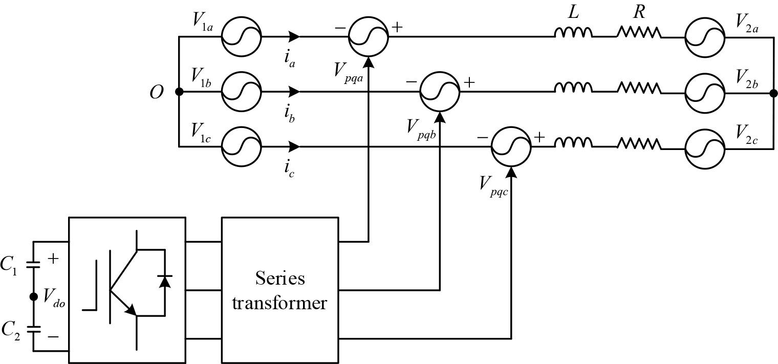
D-UPFC technology is the application of UPFC in a distribution network, which is a derivative of UPFC. The concept of UPFC is a kind of hybrid flexible AC transmission system (FACTS) equipment with an integrated series-parallel voltage source converter (VSC), which is composed of a static synchronous compensator (STATCOM) on the shunt side and static synchronous series compensator (SSSC) on the series side, and the function and structure of D-UPFC and UPFC are the same, and the working principle is also similar. D-UPFC and UPFC have the same function and structure, and the working principle is also similar. Mainly series compensation, parallel compensation, phase shift adjustment, and other functions. The difference between the two is that UPFC is used for equipment in transmission lines, while D-UPFC is suitable for equipment in the distribution network. The structure of D-UPFC can be seen in Fig. 4, and its main structure is composed of two voltage-source converters, VSC1 and VSC2, and a DC capacitor. If the current VSC1 flows to VSC2, then the process is equivalent to going through a rectification and then inversion process.

The structure of the D-UPFC
The realization of the D-UPFC function must depend on a good control strategy. Regarding the control strategy of D-UPFC, experts and scholars have done much research since the original amplitude-phase control to the development of fuzzy PID control and intelligent control in recent years. Among the many control schemes of D-UPFC, cross-decoupling, cross-coupling, multi-objective coordinated control, etc., have been verified and applied through simulation and experiment. In this paper, according to the needs of the implementation of the flexible interconnection project of a medium voltage distribution network, the series-type D-UPFC is applied to the control system to realize the fast MPC control of D-UPFC based on current feedback.
The mathematical model of the D-UPFC series side is constructed as follows:
The D-UPFC series side transformer is essentially a PWM converter that can operate in four quadrants. By equating it to a controllable voltage source, the line current can be dispatched by simply adjusting the voltage amplitude and phase angle.
The principle of the converter is shown in Fig. 5, where
The mathematical model in the transformed
Let
In a real circuit,
From there, there is:
Schematic diagram of the series converter
From Eq. 2, when line resistance
In order to verify the effectiveness of this paper’s multi-model optimization method based on the flexible interconnection engineering of MV distribution networks and the effectiveness of the voltage control strategy. In this paper, the waveform quality of the output voltage of the flexible interconnection engineering device is studied in accordance with the national standard. According to the actual situation of the device control system build a control model and simulation verification of the model. The impedance amplitude-frequency characteristics of current inner-loop control are compared in Fig. 6. The current inner-loop control system is based on capacitor current feedback, the feedback quantity contains the perturbation quantity of load current, and the response speed of the inner-loop control is generally higher than that of the voltage outer-loop. Therefore, the perturbation quantity of the load current can be effectively suppressed before it affects the output voltage, so the addition of the current inner-loop control based on capacitor current feedback can improve the dynamic performance of the system.
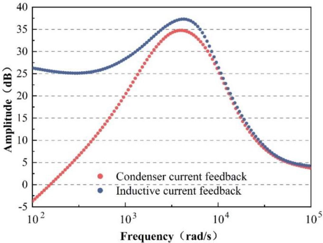
Contrast of current internal ring control impedance amplitude frequency
The waveforms of output voltage and current instantaneous values and RMS voltage waveforms are shown in Fig. 7, (a) ~ (c) are output voltage, output current and RMS voltage, respectively, where the lines of different colors represent different phases. The RMS value of the output voltage line voltage is 10kV after the interconnection device starts operation, which is consistent with the set value. When the rated load is suddenly added for 0.1 seconds, the voltage appears to fall briefly, and the voltage fall limit amplitude is 0.155 pu, duration 5ms, and then quickly recovers to the set voltage command value. Therefore, by adopting the control strategy discussed in this paper, the output voltage of the device has better dynamic characteristics and steady-state accuracy, and can meet the requirements of the distribution network for voltage quality.

Output voltage current waveform and voltage effective value waveform
The voltage fluctuation of the load side of the grid voltage is shown in Fig. 8. The amplitude of the grid voltage changes abruptly to 0 V when t is about 0.20 s, and then the grid voltage returns to normal when it is about 0.27 s. At this time, the load-side voltage output is stable, and it can realize the normal power supply requirements for the load.
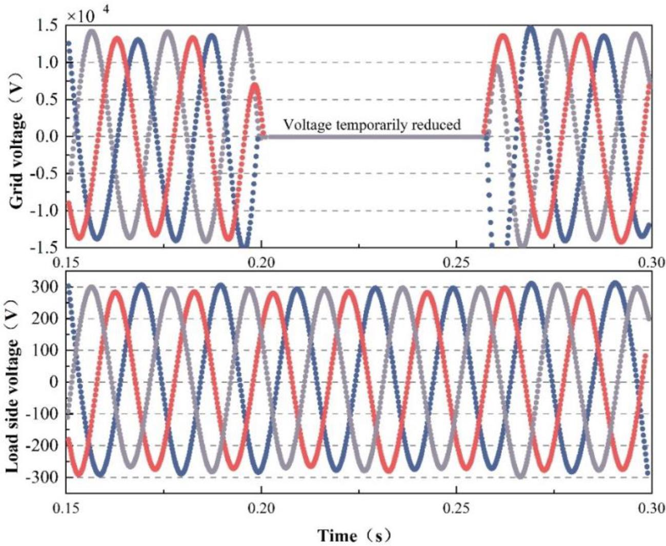
The voltage fluctuation of the voltage of the grid voltage load
In the power unit DC bus voltage waveform shown in Figure 9, in 0.20s, the grid voltage amplitude suddenly changed to 0V. At this time, the power unit DC bus voltage is reduced to 690~720V, the grid storage battery pack terminal voltage is higher than the DC bus voltage, and the storage battery pack through the power diode is automatically put into operation to maintain a constant DC bus voltage, to ensure the load continues to be reliable power supply.
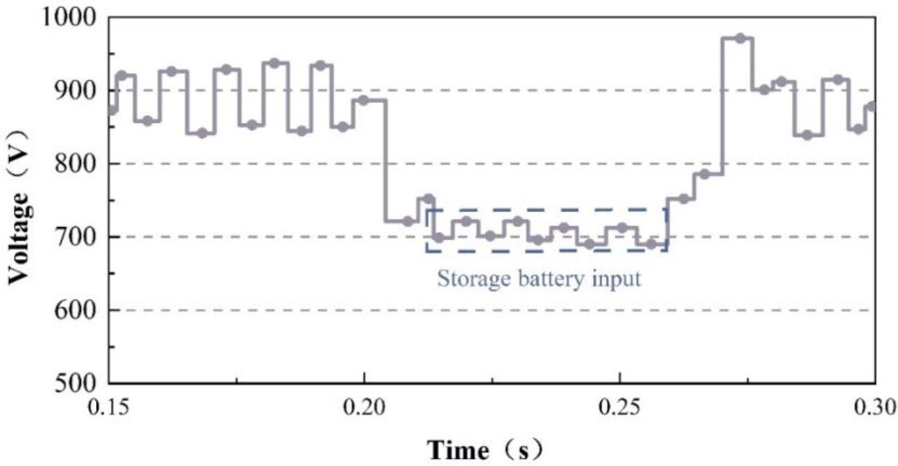
Power unit dc bus voltage waveform
In this paper, the effects of three typical control strategies of current inner-loop control, voltage outer-loop control and power outer-loop control are set up, which are denoted as Scheme1~3 (Scheme1~3). The optimization is carried out using the method of this paper, and the objective functions such as system operating cost, network loss and voltage deviation are solved by using the forward back generation method of current calculation. The effectiveness of different control operation strategies is verified by comparing the results.
The comparative results of the operation of different strategies are shown in Table 1. The three typical control strategies of current inner-loop control, voltage outer-loop control and power outer-loop control are all more effective than the traditional initial system. Although the operation cost of scheme 1 is the lowest at 1559.5yuan, the voltage deviation and the total active network loss throughout the day are relatively high compared to both scheme 2 and scheme 3. It shows that although the current inner-loop control strategy has a lower operating cost and can provide reactive power compensation, it cannot respond quickly to the system’s reactive power changes and compensate a continuous amount of reactive power compensation to the current grid, and due to the limited regulation capability, it cannot meet the requirement of accurate real-time operation optimization for renewable energy with strong uncertainty.
The performance of different policies is the result of the comparison
| Scheme | Operating cost/CNY | Voltage deviation/p.u. | Total work loss/kWh |
| Initial system | — | 0.0870 | 4865.45 |
| Scheme 1 | 1559.5 | 0.081 | 3332.0 |
| Scheme 2 | 5543.8 | 0.0746 | 2897.3 |
| Scheme 3 | 3696.1 | 0.0685 | 2655.2 |
The voltage deviation and the total active network loss of the whole day of scheme 2 are better than scheme 1, but the system operation cost expense is higher for 5543.8 Yuan.The voltage deviation and all-day total active network loss of scheme 3 systems are reduced by approximately 21% and 46%, respectively, compared to the initial system. Compared with scheme 2, the voltage deviation is reduced from 0.0746p.u. to 0.0685p.u., and the total active network loss for the whole day is reduced from 2897.3kWh to 2655.2kWh, which shows that under the power outer loop control, it is able to reduce the operation cost while maintaining the stability of the system power quality.
The comparison of grid improvement under different strategies is shown in Fig. 10, where 35 nodes of different control strategy schemes at the same moment are selected for comparison, and it can be seen that the voltage of the grid is improved differently under the three control strategies, and all of them have the role of regulating the power quality. Among them, the voltage improvement of scheme 3 is the best, and the voltage is up to 0.997 p.u., which indicates that the regulation of system reactive power changes under power outer-loop control complements and influences each other. Therefore, the use of a power outer loop control strategy better meets the operational requirements of the system, which need to take into account the system’s power quality, operating economy, and response speed.
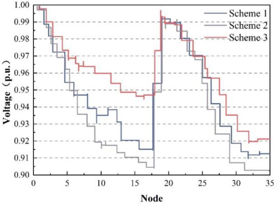
Contrast to grid improvements under different strategies
In order to verify the practical application effect of the flexible interconnection project in this paper, taking K province as an example, based on the real data of the power grid for the line load distribution in the region, and to alleviate the problems of line heavy load and PV back-feeding, three flexible interconnection devices are constructed to realize the flexible interconnection of the 10kV south line (A), spring line (B), and river line (C), and the coordinated control device monitors and regulate the trend of the three 10kV lines in terms of heavy load and back-feeding power to optimize the adjustment of line power and solve the problem of heavy load operation. Through the coordinating control device, the three 10kV lines are monitored to optimize the adjustment of line power, solve the problem of heavy load operation, and transfer the back-feeding power from the South Line and the Jiang Line to the Spring Line which is not back-feeding during the time of large PV output, so as to equalize the back-feeding loads, reduce the back-feeding spikes, solve the problem of terminal voltage overrun and enhance the capacity of regional PV consumption.
The interconnection project’s application has a comparative effect that is shown in Fig. 11, with Figs. (a) and (b) showing the effect before and after the application, respectively. From the measured power curve, it can be seen that from June 30 to July 5, under the coordinated control of the flexible interconnection engineering implementation in this paper, the maximum load of the three lines can be controlled by 2.5 MW, cutting down the load spikes by 20%, and the FIDs of the three lines are all in the range of -1~1, and the heavy loads of the 10 kV south line (A) and spring line (B) are effectively alleviated to ensure the safe operation of the distribution network. It is proved that the flexible interconnection technology can effectively improve the power supply reliability of the lines, can effectively solve the problems of feeder heavy load and PV back-feeding in the distribution network, improve the power supply efficiency of the distribution network, and provide a strong guarantee for the local consumption of a high proportion of distributed new energy.
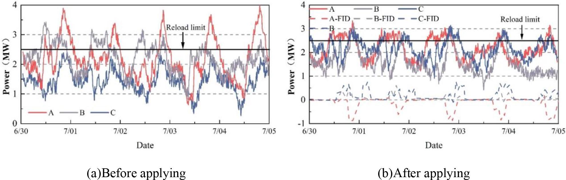
The comparison effect of the Internet engineering application
In this study, based on the flexible interconnection project, the multivariate model optimization of the distribution network was implemented using B2B VSC, MMC-type B2B VSC and D-UPFC technologies, and the following conclusions were drawn based on the experimental results:
The output voltage line voltage RMS value of 10kV after the interconnection device starts operation is consistent with the set value. When the rated load is added abruptly for 0.1 seconds, the voltage appears to fall briefly, and the limit amplitude of the voltage fall is 0.155 pu for 5 ms, and then it quickly recovers to the set voltage command value. The amplitude of the grid voltage suddenly changes to 0V, and the power unit DC bus voltage decreases to 690~720V in about 0.27s. When the grid voltage returns to normal, the terminal voltage of the grid storage battery pack is higher than the DC bus voltage. Comprehensive description of the control strategy in this paper: the device output voltage has better dynamic characteristics and steady-state accuracy to meet the distribution network requirements for voltage quality and, at the same time, can realize the normal power supply requirements for the load to ensure that the load continues to be reliable power supply. The voltage deviation and all-day total active network loss of the scheme 3 system are reduced by about 21% and 46%, respectively, compared with the initial system. In the comparison of different control strategy schemes, the voltage improvement of Scheme 3 is the best, and the voltage can reach up to 0.997 p.u., which indicates that the regulation of system reactive power changes under power outer-loop control complements and influences each other. Therefore, the use of a power outer-loop control strategy better meets the system needs to take into account the power quality, operating economy, and response speed requirements of the operational requirements. The maximum load of the three lines after the flexible interconnection project should be able to control 2.5MW, cutting the load peak by 20%. Meanwhile, the FID of all three lines is controlled between -1 and 1. It shows that the heavy load situation of the lines has been effectively alleviated, and the safe operation of the distribution network is guaranteed.
This project is supported by the 2024 Science and Technology Project of State Grid Gansu Electric Power Company: Research on Key Technologies and Typical Configuration of Flexible Interconnection in Medium Voltage Distribution Networks (No. B72703241203).