Social network analysis of the casual community: identifying key players and network structure

Publié en ligne: 17 mars 2025
Reçu: 21 oct. 2024
Accepté: 11 févr. 2025
DOI: https://doi.org/10.2478/amns-2025-0159
Mots clés
© 2025 Bo Ma, published by Sciendo
This work is licensed under the Creative Commons Attribution 4.0 International License.
Wushu Sanshou, with a long history, is a form of human movement condensed by the Chinese people in the long-term labor practice and struggle for life, which is attributed to Chinese traditional sports. Wushu is the most direct form of technical expression of Wushu sports [1-4]. Sanshou is two people in accordance with certain rules, under certain conditions. It is a modern competitive sport of unarmed confrontation using kicking, punching, wrestling and defense techniques in Wushu [5-7]. It is an old and young sport, a modern competitive sport with both strong oriental national cultural characteristics and commonality of western competitive sports. The sparring community, on the other hand, is a social organization focusing on combat sports, including sparring, boxing and other forms of sports [8-11].
Social network analysis is a quantitative research method used to describe and explain the relationships between individuals in a social system. Through social network analysis, in social networks, individuals can be people, organizations, countries, etc [12-14]. Nodes represent individuals, and edges represent relationships between individuals, such as friendship, cooperation, information flow, etc. Social network analysis focuses on studying the structure and pattern of the whole network, as well as the position and role of nodes in the network [15-17]. Social network analysis can reveal the relationship between individuals, the structure and pattern of the network, and provide theoretical support for the operation and optimization of the social system. Its application in casual communities is conducive to the creation of harmonious community relations. However, social network analysis also has its limitations and needs to overcome challenges such as the difficulty of data collection and privacy protection issues [18-21].
Social network analysis focuses on emphasizing the connections between each actor and other actors, as well as their influence on each other.In this paper, 23 students from a college’s casual sparring community are selected as the research subjects, and the network structure of this community is visualized through social network analysis.Firstly, density, distance, centrality, and other relevant indicators, such as the overall network characteristics of the casual sparring community, are selected to identify key participants. Then, the groups were divided into cohesive subgroups to explore the relationship that exists between key participants and each member.
A specific network can choose between two modes of describing the relational data it obtains, diagrams and matrices, but there are advantages and disadvantages to each of these methods.Diagrams provide the reader with a more intuitive representation of the structure of the network, but they lack mathematical tractability. In contrast, although matrices do not appear to have a sufficiently reader-friendly interface, they are very convenient for performing complex mathematical and computer analyses of social network data [22].
The following is a practical example of a graphical representation of a network, a network can be represented as a graph
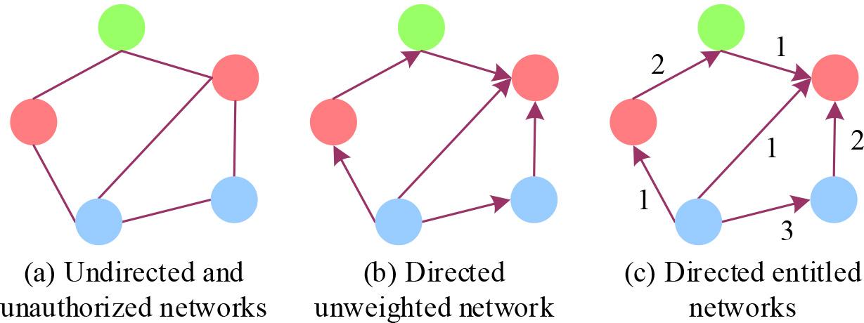
Different types of networks
Degree.
The node degree, denoted
Average Distance
For an undirected graph, there are many cases of node
The average path length L of the network is defined as the average of the distances between any two nodes, i.e.
The above equation includes the path from the node to itself (this path is always 0), the average path length of a network reflects the degree of aggregation of a network, the average path length of a network is long (through how many nodes are linked together), the network has a high degree of aggregation, and the recent research on complex networks has found that, despite the size of the complex network
Network Density
Density describes how closely the points in a graph are related to each other. A “complete graph” (called a perfect graph in graph theory) is a graph in which all the points are connected, and this kind of completeness is very demanding and is only possible in very few small network graphs. The notion of density is an attempt to assess the completeness of a graph, and it is clear that the closer a network is to this completeness, the greater its density, and vice versa, and the density also reflects the overall level of cohesion of a graph. The general idea is that the more connections between nodes in a graph, the denser the graph is, indicating that the nodes represent closer relationships between network members [23].
There are various techniques and methods for describing networks in social network analysis, with network diagrams and matrices being the most basic descriptive methods.
Representation of diagrams
For the graph Social networks have a relationship diagram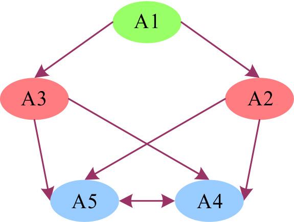
Representation of the matrix
A matrix is a representation of the nodes in a network graph into rows and columns, with 0’s and 1’s used to represent the relationships between the nodes. For example, the directed graph of Fig. 2 can be represented in the form of Table 1. Table 1 is a positive square matrix, (A1, A2) = 1 means that A1 to A2 is connected and is A1 pointing to A2, (A1, A5) = 0 means that there is no connection between A1 and A5.
Matrix form of figure 2
A1
A2
A3
A4
A5
A1
0
1
1
0
0
A2
0
0
0
1
1
A3
0
0
0
1
1
A4
0
0
0
0
1
A5
0
0
0
0
1
Point-degree centrality is a metric that quantifies centrality based on the degree of a node in a graph.
Point Centrality
“Point centrality” is the simplest and most intuitive indicator, which describes the degree to which a node is located in the “core” position in the graph, portraying the ability of the point to develop relationships with other points in the graph.
Point centrality is divided into absolute point centrality and relative point centrality, and the absolute point centrality of point
Point
Pointwise central potential
The “point degree central potential” describes the central tendency of the whole graph, i.e. the tendency of whether there is a core node in the graph.
The derived idea of the central potential indicator is: first find the maximum value of the centrality of all nodes in the graph; then calculate the difference between this maximum value and the centrality of all other nodes, and find the sum of these differences; and finally use this sum to remove the maximum possible value based on the sum of the above differences. The formulae are described as follows:
If the pointwise centroid potential is described in terms of absolute pointwise centroid degrees, it takes the form:
If the pointwise centroid potential is described in terms of relative pointwise centrality, it takes the form:
Here
Intermediate centrality is a metric that quantifies centrality based on the number of geodesics in a pair of nodes in a graph.
Intermediate Centrality
“Intermediate centrality” describes the extent to which a node acts as an “intermediary” (or “bridge”), and it portrays the ability of that point to control interactions between other points in the graph.
Median centrality is further divided into absolute and relative median centrality. Assuming that the number of geodesics existing between points
The absolute median centrality of a point
The relative median centrality of a point
Relative intermediate centrality is commonly used for calculations.
Intermediate Centrality
The “intermediate centrality potential” describes the intermediate trend of the whole graph, i.e., the trend of whether there is an “intermediary” node in the graph.
It is proved that the absolute intermediate centrality is used to describe the intermediate central potential in the form of:
The intermediate central potential is described in terms of relative intermediate centrality in the form:
Here
Proximity to centre
“Proximity to centre” describes the distance between a point and all other points in the graph. If the distance between the point and all other points in the graph is very short, it means that the point is “close” to all other points in the graph, i.e., the proximity to centre of the point is very high. This means that the proximity centrality of the point is high. Proximity centrality portrays the ability of a point to escape from the control of other points in the graph, and an actor in a network has a high proximity centrality if they are less dependent on others in their interactions with other actors.
Proximity centrality is further divided into absolute proximity centrality and relative proximity centrality. The absolute proximity centrality of point
The relative proximity centrality (denoted as
Relative proximity to centrality is commonly used for calculations.
Proximity Centrality Potential
The “proximity centrality potential” describes the proximity trend of the entire graph, i.e., the tendency of the graph to have a node with a short distance from all other points.
It is proved that the proximity centrality potential is described by the relative proximity centrality degree in the form of
Here
The faction method, which utilizes the CPM faction filtering algorithm, is the method used in this paper to analyze cohesive subgroups. In the actual research cooperation network, as the cooperation relationship between research members continues to expand and deepen, a research member may belong to multiple small groups, i.e., they exist in multiple cohesive subgroups, then this individual’s position in the group is undoubtedly important, and the CPM algorithm is able to find such overlapping structures between cohesive subgroups [24].
A faction is a set where any two points are connected, i.e., a complete subgraph. Within subgroups, nodes are highly connected and prone to form factions, while edges between subgroups are less likely to form larger complete subgraphs. Thus subgroups can be discovered by finding out the factions in the network. K-factions are defined as complete subgraphs that have k nodes in the network, and when a k-faction overlaps with another k-faction by k-1 nodes, it is considered connected.Some nodes in the network may exist in more than one k-faction subgroup, so we can discover the overlapping structure between the groups using this algorithm. k as an input parameter may affect the subgrouping result, but the experiment proves that the effect is small, and it generally takes the value of 4-6. Therefore, in this paper it is set to 4.
We mine cohesive subgroup metrics from three perspectives: based on relationships between cohesive subgroups, based on relationships within cohesive subgroups, and based on relationships between cohesive subgroups and the overall network.
Based on the relationship between cohesive subgroups, metrics
Mean value of intermediate centrality of subgroup overlap points For the relationship between cohesive subgroups, there exists a portion of nodes that belong to multiple cohesive subgroups and have highly close cooperation with any of these cohesive subgroups. These nodes must possess a strong ability for information communication, resource transfer, and knowledge circulation. Therefore, we use intermediate centrality to quantify this ability of theirs, and the calculation method uses relative value. Mean value of proximity centrality of subgroup overlap points The importance of the nodes in the overlapping part of the cohesive subgroups is self-evident, so whether they are able to promote the flow of information in the research cooperation network, this part is to use the degree of proximity to the centre of the portion to portray this characteristic, that is, in addition to the role of communication and coordination intermediary between the cohesive subgroups in which they are located, whether they are able to control the resources for the other nodes or cohesive subgroups, and how much the control of the resources, the significance of this indicator is The practical significance of this indicator lies in the portrayal of whether the members located outside the subgroups have access to sufficient information and opportunities for scientific cooperation.
Indicators based on relationships within cohesive subgroups
Mean value of subgroup clustering coefficient The cohesive subgroups, which are small groups in the network, can be understood as sub-networks in the network. Then, the sub-networks also have the same nature as social networks, so this part uses the clustering coefficients to portray the cooperation tightness within each cohesive subgroup, and the mean value of subgroup clustering coefficients is taken as one of the indicators of the performance impact. Mean value of co-operation intensity within sub-clusters The clustering coefficient of subgroups only takes into account the degree of the node.That is, it only considers the number of times cooperation occurs within the subgroups and ignores the role of cooperation intensity on performance. Therefore, the mean value of cooperation intensity within subgroups is used as one of the examined indicators of influencing the performance of the scientific research team, and in this part, we deal with the intensity of cooperation within subgroups as the ratio of the sum of the weights of the edges within a subgroup to the number of nodes of the subgroups.
Indicators that are based on the relationship between cohesive subgroups and the overall network
Number of cohesive subgroups The number of subgroups in the network represents how the connections between individual members of the research team are formed to form the overall network. Mean value of cohesive subgroup members Some related studies have shown that there is a correlation between team size and performance, so as a large team within the small group size and team performance whether there is also a certain relationship between, this paper will be cohesive subgroup member mean value as one of the indicators of verification. Percentage of cohesive subgroups exceeding the mean value of size In social network relationships, the number of cohesive subgroups varies, and the number of members within each cohesive subgroup varies. In contrast, Palla, Pollner, and Barabási et al. study the analysis of the association structure of collaborative networks of scientists and networks of mobile phone users and find that large subgroups that have a dynamically changing internal membership can instead sustain the subgroups for a longer period of time. In contrast, smaller subgroups should be maintained as long as possible relatively fixed in terms of personnel to maintain stability. According to this idea, the distribution of large sub-subgroups in the network will also have an impact on performance, then this part uses the cohesive subgroup percentage beyond the scale average to verify the relationship between it and team performance. Mean value of cohesive subgroup density The cohesive subgroup density is mainly used to describe the phenomenon of small groups in the social network, and the closer its value is to 0, the it indicates that the relationship of small groups within a large group tends to be randomly analysed, and there is no factionalism in the situation. We obtain this indicator by calculating the density of each cohesive subgroup and then finding the average value.
Social network analysis tends to see members of the sports community as a part of a particular network of relationships.The scope of the survey is known as the parent boundary in the network, in the closed network, to take the entire group to administer the test to collect information. In order to facilitate the research, this paper selected the X University of Sanshou community as the research object. There are 23 people, martial arts coaches, teacher workers, student positions, etc., the use of questionnaires. The research object is divided into 3 groups. Questionnaires issued 23 copies, a valid questionnaire with 23 copies, and a recovery rate of 100 per cent.
Based on the statistical results of the number of community members choosing and being chosen in the questionnaire survey of interpersonal relationships, the overall social network diagram of the relationship between members of the casual community was drawn, as shown in Figure 3. Through the network diagram, it is possible to comprehend the network structure and group characteristics of the inner members.From the overall network structure, the structure is relatively close. The members constitute an organic whole, there is no lone member (i.e., there is no member in the community who does not contact others and is not contacted by others), and it can reflect more interpersonal interaction and stronger cohesion within the community. The No. 1 member is in the centre of the overall network, and the extent of the network has the greatest degree of centrality, and it also has a greater influence on the development of the community; Members #3, #8, #9, #17, and #20 are the more active members of the network and have a higher number of connected members, they initiate contact with other members or are constantly nominated and selected by other members, these members are more active in the association network. The other members are less active within the association, and member #6 has only one inward relationship connection and no outward relationships.
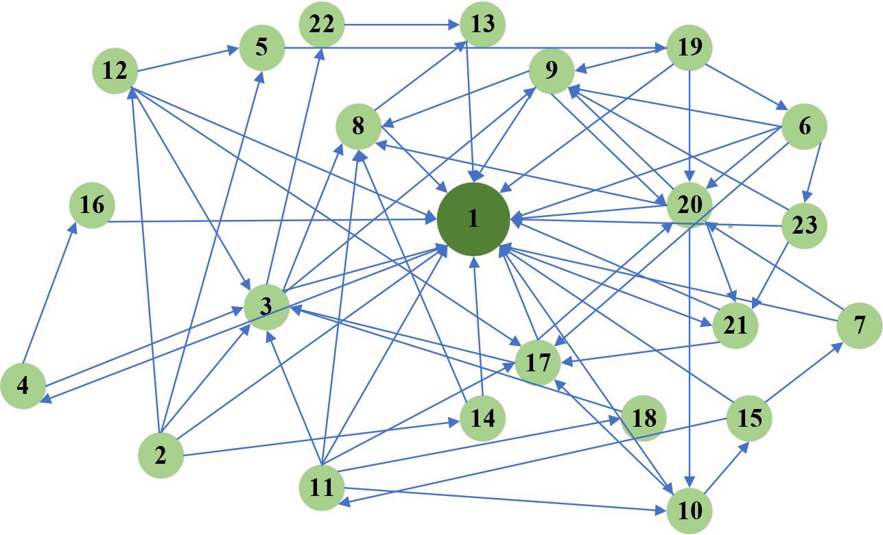
The overall network structure diagram of the community members
In casual communities, relationships between members are established and maintained through forms of interaction.The shortest distance between members within a community’s membership network is interaction distance, which reveals the directness and indirectness of the connections between them. If there is a direct connection between two members, the interaction distance value is 1. If there is no direct connection between two members and they need to be connected through an intermediary member, the interaction distance value is 2. If they need to be connected through two intermediaries, the interaction distance value is 3, and so on. Table 2 displays the results of the UCINET software calculations, which can be used to obtain the average interaction distance and association cohesion values.
The overall network interpersonal interaction distance analysis
| Loose beat community | Average interaction distance | Community cohesion |
| First set | 1.542 | 0.388 |
| Second group | 1.735 | 0.314 |
| Third group | 4.212 | 0.152 |
From the table illustration, the interaction and interaction between the casual community members of the first and second groups needs to have nearly two intermediaries to pass on average. In comparison, the interaction and interaction between the casual community members of the third group need more than three intermediaries to establish a connection, which indicates that the members of the third group are easy to get acquainted with each other. However, the average interaction distance still requires more than three intermediaries to be passed on, and the overall interaction between the casual community members of the third group is infrequent. Frequent, and the interaction awareness is relatively weak.
Emotional network analysis
The affective network is mainly reflected in the degree of emotional intimacy that exists between the members of the community network, which can affect the interpersonal harmony and development of the sparring community. The emotional network of the members of the sparring community is shown in Figure 4. In the figure, it can be seen that members 22 and 18 and members 16 and 23 are two isolated groups in the affective network, and they are emotionally connected two by two and have no connection with other members of the community. The remaining members form a larger, more closely related affective network with each other (subfigure), in which the central figures are members #10 and #14.
Community affective network map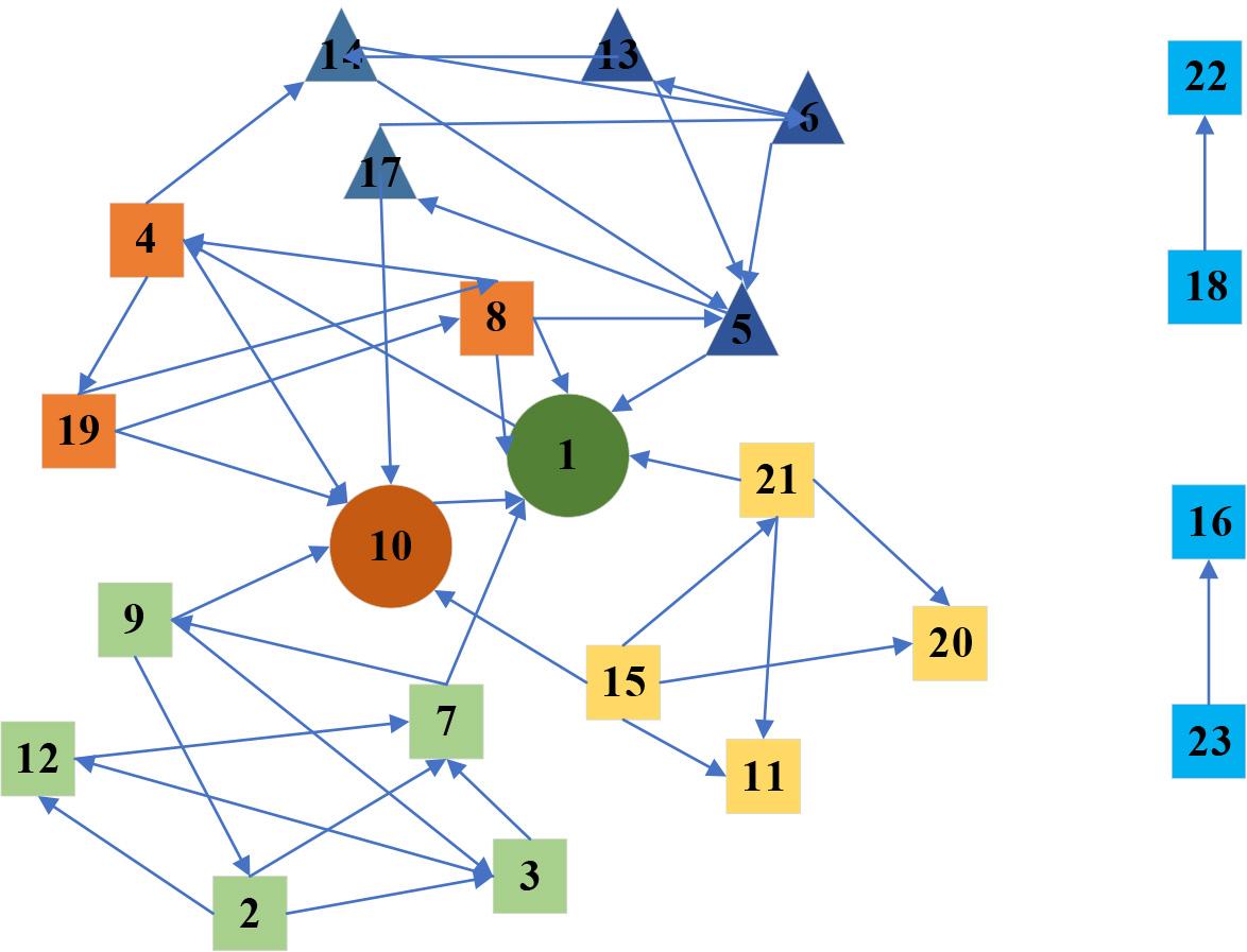
Information network analysis
The information network in this study is mainly formed by the transmission of information (messages, news, etc.) constructed from the interpersonal interactions of the members of the Sanshou community. The information network of the members of the Sanshou community in University X is shown in Figure 5. As can be seen from the figure, the dissemination of relevant information within the sparring community covers all members of the community, which is conducive to the development of the community as well as the management of ideas instilled into the brain of each member. Member 9 is at the core of the information network, and members 11, 18, 21, and 23 are connected to a larger number of other members who are more capable of controlling the flow of information, and who have a greater influence on the development of the community. Members #1 and #7 and #14 have less information coming to them and are at the periphery of the information network.
Information network diagram for community members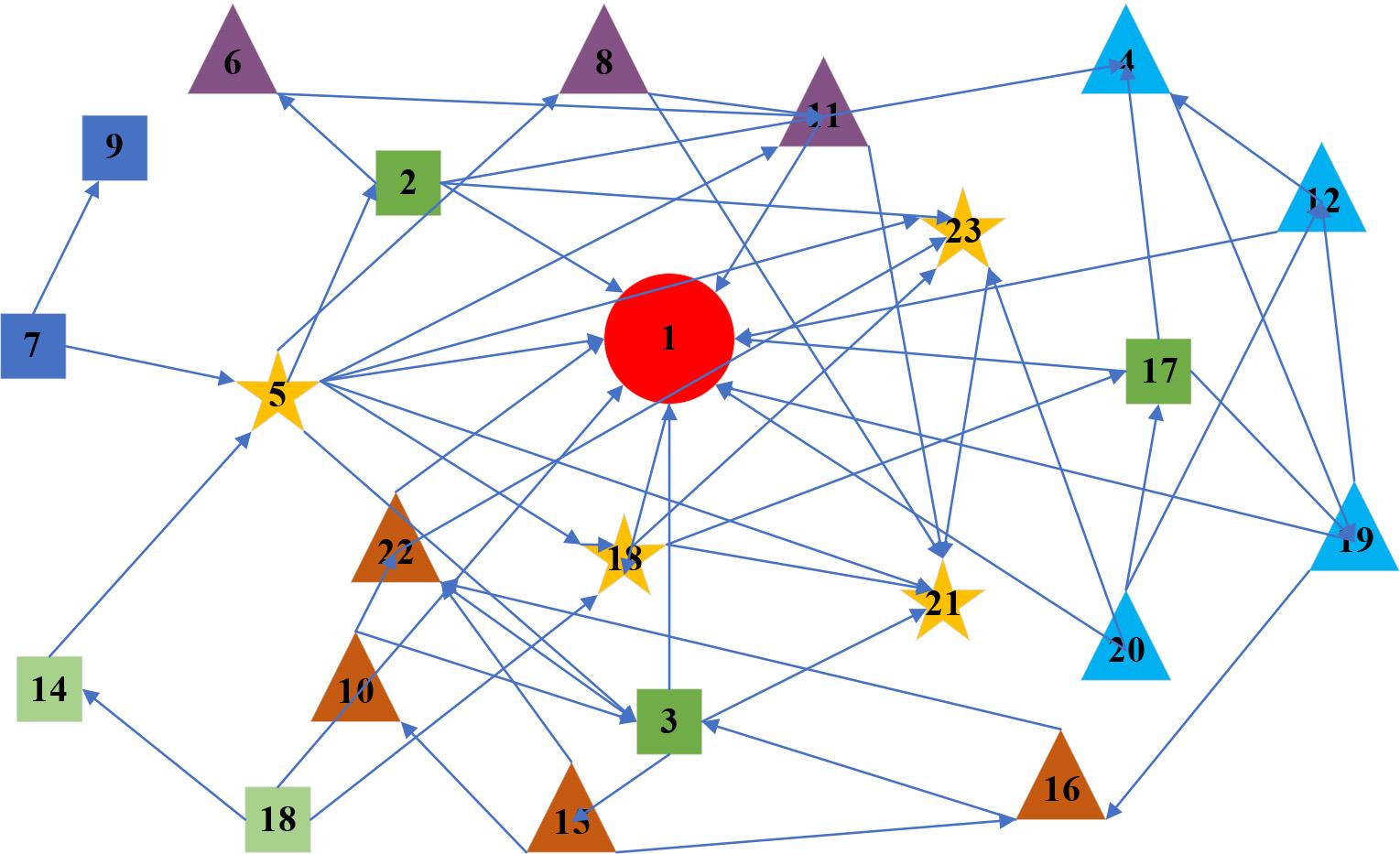
Analysis of technical counselling network
In the consulting relationship network, members who are good at Sanda martial arts are more likely to be in the centre of the network than those who are poor in skills, those who are willing to help others are more likely to be chosen by other members, and those who are extroverted are better than those who are introverted, and those who are extroverted are usually more expressive, which makes it easier for them to be the intermediary of the flow of information in the community and the bridge. The technical counselling network of the casual sparring community is shown in Figure 6. From the figure, it can be seen that the technical counseling network of the loose-knit community is relatively sparse, and the members who are at the core of the network are mostly No. 5, No. 7, No. 11 and No. 17.
Community members technical consulting network
In the social network of casual community members, if the neighbouring members of a member are the core members of the network, the member will be in a more central position in the network compared to other members. Therefore, by analysing the centrality of the eigenvectors of the overall members, we can obtain the members who are in the core, middle and edge positions in the overall network structure, and the results of the analysis are shown in Table 3. After measuring the centrality of the overall members’ eigenvectors, it is found in the order of centrality that #1 occupies the first place in the centrality of the 3 relational network eigenvectors of 0.59, 0.65 and 0.73, respectively. It indicates that in the casual community, No.1 has a large number of important nodes and a prominent position and is at the centre of the whole network, playing a decisive role in the process of information flow and interaction, and being able to control members’ emotions, social information and other resource flows. Describe the dominant role that member 1 plays in the usual activities. In a community organization, member 1 is responsible for most of the community’s work, including organizing entries, costume selection, equipment management, conflict mediation between members, and so on. Within the team, the captain is the most vocal person who has a high level of voice.
The relative eigenvector center of the three dimensions
| Affective communication | Information transfer | Technical consultation | ||||||
| Member | Eigenvec | nEigenvec | Member | Eigenvec | nEigenvec | Member | Eigenvec | nEigenvec |
| 1 | 0.59 | 56.06 | 1 | 0.65 | 63.23 | 1 | 0.73 | 71.6 |
| 2 | 0.59 | 55.99 | 2 | 0.64 | 61.57 | 2 | 0.72 | 61.32 |
| 3 | 0.3 | 15.6 | 3 | 0.32 | 16.81 | 3 | 0.4 | 11.5 |
| 4 | 0.42 | 31.89 | 4 | 0.36 | 22.95 | 4 | 0.44 | 11.5 |
| 5 | 0.39 | 28.74 | 5 | 0.41 | 29.61 | 5 | 0.49 | 23.77 |
| 6 | 0.39 | 27.9 | 6 | 0.32 | 16.81 | 6 | 0.4 | 11.5 |
| 7 | 0.39 | 28.54 | 7 | 0.32 | 16.81 | 7 | 0.4 | 49.71 |
| 8 | 0.38 | 26.47 | 8 | 0.45 | 35.92 | 8 | 0.53 | 68.89 |
| 9 | 0.39 | 28.38 | 9 | 0.36 | 22.62 | 9 | 0.44 | 13.41 |
| 10 | 0.39 | 28.9 | 10 | 0.32 | 17.06 | 10 | 0.4 | 9.34 |
| 11 | 0.31 | 16.28 | 11 | 0.36 | 22.95 | 11 | 0.44 | 20.51 |
| 12 | 0.42 | 32.24 | 12 | 0.3 | 13.56 | 12 | 0.38 | 5.88 |
| 13 | 0.42 | 32.03 | 13 | 0.34 | 19.62 | 13 | 0.42 | 23.25 |
| 14 | 0.35 | 22.41 | 14 | 0.45 | 35.67 | 14 | 0.53 | 14.35 |
| 15 | 0.34 | 21.27 | 15 | 0.42 | 30.73 | 15 | 0.5 | 24.97 |
| 16 | 0.4 | 29.03 | 16 | 0.3 | 13.8 | 16 | 0.38 | 16.17 |
| 17 | 0.3 | 15.27 | 17 | 0.24 | 5.13 | 17 | 0.32 | 8.65 |
| 18 | 0.34 | 21.17 | 18 | 0.48 | 38.91 | 18 | 0.56 | 5.97 |
| 19 | 0.3 | 15.3 | 19 | 0.32 | 16.81 | 19 | 0.4 | 16.98 |
| 20 | 0.31 | 16.75 | 20 | 0.39 | 26.9 | 20 | 0.47 | 17.07 |
| 21 | 0.3 | 14.98 | 21 | 0.29 | 12.42 | 21 | 0.37 | 2.76 |
| 22 | 0.46 | 37.91 | 22 | 0.55 | 49.87 | 22 | 0.63 | 27.77 |
| 23 | 0.39 | 27.73 | 23 | 0.32 | 16.52 | 23 | 0.4 | 13.76 |
With the help of the software UCINET, after calculating the point degree centrality of the members of the casual community and finding the different relationship dimensions, the point-in and point-out status presented among the members varies. The results of the analysis are shown in Table 4. In terms of the affective relationship network, members 1, 10 and 13 ranked in the top three in terms of points and had a good point-out degree, which indicates that they have good effective communication with other members within the organisation and informally influence others. By calculating the distance between the members, it was found that each member has a certain number of intermediate groups, and their distribution is basically in line with the power law. In the information exchange network, the higher degree of entry is Member 1, member 12, and Member 2, and the relatively higher is Member 5, Member 9, and Member 20. These members, due to the possession of information and knowledge in the organisation, become the primary target for others to take the initiative to ask for advice and contact and belong to the scattering node in the directionless network.
A list of points of point center for community participants
| Affective communication | Information transfer | Technical consultation | ||||||||||||
| Member | OD | ID | NOD | NID | Member | OD | ID | NOD | NID | Member | OD | ID | NOD | NID |
| 1 | 17 | 22 | 50.73 | 61.6 | 10 | 12 | 22 | 31.72 | 64.95 | 13 | 26 | 6 | 12.33 | 1.42 |
| 12 | 13 | 25 | 36.93 | 71.95 | 7 | 11 | 6 | 28.27 | 9.78 | 5 | 13 | 6 | 6.73 | 1.42 |
| 2 | 10 | 10 | 26.59 | 20.22 | 18 | 9 | 5 | 21.37 | 6.33 | 1 | 12 | 29 | 6.3 | 11.34 |
| 16 | 10 | 8 | 26.59 | 13.33 | 11 | 8 | 8 | 17.92 | 16.67 | 15 | 11 | 5 | 5.87 | 0.99 |
| 8 | 10 | 8 | 26.59 | 13.33 | 8 | 8 | 4 | 17.92 | 2.88 | 10 | 9 | 6 | 5.01 | 1.42 |
| 5 | 9 | 9 | 23.14 | 16.77 | 19 | 7 | 7 | 14.48 | 13.23 | 18 | 8 | 6 | 4.57 | 1.42 |
| 17 | 9 | 12 | 23.14 | 27.12 | 2 | 7 | 5 | 14.48 | 6.33 | 21 | 7 | 4 | 4.14 | 0.56 |
| 6 | 9 | 9 | 23.14 | 16.77 | 16 | 7 | 8 | 14.48 | 16.67 | 14 | 7 | 6 | 4.14 | 1.42 |
| 10 | 9 | 10 | 23.14 | 20.22 | 15 | 7 | 5 | 14.48 | 6.33 | 6 | 7 | 4 | 4.14 | 0.56 |
| 14 | 9 | 11 | 23.14 | 23.67 | 5 | 7 | 7 | 14.48 | 13.23 | 16 | 7 | 8 | 4.14 | 2.28 |
| 20 | 8 | 9 | 19.69 | 16.77 | 1 | 7 | 5 | 14.48 | 6.33 | 19 | 7 | 4 | 4.14 | 0.56 |
| 11 | 8 | 14 | 19.69 | 34.01 | 4 | 7 | 4 | 14.48 | 2.88 | 2 | 7 | 12 | 4.14 | 4.01 |
| 18 | 8 | 6 | 19.69 | 6.43 | 6 | 6 | 5 | 11.03 | 6.33 | 3 | 6 | 5 | 3.71 | 0.99 |
| 4 | 8 | 8 | 19.69 | 13.33 | 13 | 6 | 15 | 11.03 | 40.81 | 9 | 6 | 5 | 3.71 | 0.99 |
| 15 | 8 | 8 | 19.69 | 13.33 | 3 | 6 | 23 | 11.03 | 68.4 | 22 | 6 | 4 | 3.71 | 0.56 |
| 7 | 8 | 16 | 19.69 | 40.91 | 8 | 6 | 7 | 11.03 | 13.23 | 11 | 6 | 5 | 3.71 | 0.99 |
| 21 | 7 | 5 | 16.24 | 2.98 | 9 | 6 | 5 | 11.03 | 6.33 | 12 | 6 | 4 | 3.71 | 0.56 |
| 3 | 7 | 6 | 16.24 | 6.43 | 12 | 6 | 5 | 11.03 | 6.33 | 17 | 6 | 5 | 3.71 | 0.99 |
| 22 | 7 | 6 | 16.24 | 6.43 | 15 | 6 | 4 | 11.03 | 2.88 | 20 | 6 | 14 | 3.71 | 4.87 |
| 9 | 7 | 10 | 16.24 | 20.22 | 17 | 6 | 5 | 11.03 | 6.33 | 8 | 6 | 4 | 3.71 | 0.56 |
| 13 | 7 | 5 | 16.24 | 2.98 | 22 | 6 | 4 | 11.03 | 2.88 | 7 | 6 | 5 | 3.71 | 0.96 |
| 23 | 7 | 12 | 16.24 | 27.12 | 23 | 6 | 4 | 11.03 | 2.88 | 4 | 6 | 4 | 3.71 | 0.56 |
| 4 | 6 | 9 | 12.8 | 16.77 | 21 | 6 | 4 | 11.03 | 2.88 | 23 | 5 | 4 | 3.28 | 0.56 |
This study empirically analysed the factors affecting the mediated centrality of fitness self-organisation in Fushun City using a questionnaire and structural equation modelling. The results were obtained using UCINET statistics, as shown in Table 5.
The center of the community is involved in the center of the community
| The center of the emotional network | The center of the emotional network | The center of the technical network | ||||||
| Member | Betweenness | nBetweenness | Member | Betweenness | nBetweenness | Member | Betweenness | nBetweenness |
| 2 | 240.14 | 32.85 | 1 | 260.32 | 36.28 | 5 | 278.1 | 28.64 |
| 1 | 148.54 | 21.57 | 3 | 160.32 | 21.14 | 9 | 231.48 | 23.83 |
| 23 | 68.09 | 11.66 | 5 | 121.06 | 16.8 | 2 | 127.5 | 11.97 |
| 8 | 67.13 | 11.54 | 12 | 46.28 | 6.44 | 16 | 58.21 | 5.79 |
| 10 | 29.82 | 6.95 | 19 | 36.34 | 6.11 | 11 | 41.65 | 3.59 |
| 11 | 28.39 | 6.77 | 15 | 30.44 | 4.55 | 20 | 35.44 | 3.05 |
| 21 | 25.5 | 6.41 | 21 | 20.78 | 1.78 | 19 | 27.11 | 1.9 |
| 6 | 25.36 | 6.4 | 9 | 18 | 1.55 | 21 | 20.21 | 1.3 |
| 22 | 24.3 | 6.27 | 11 | 18 | 1.11 | 15 | 11.55 | 1.12 |
| 19 | 20.21 | 5.76 | 20 | 9.45 | 1 | 14 | 3 | 0.19 |
| 14 | 19.95 | 5.73 | 4 | 9.21 | 0.98 | 17 | 2.1 | 0.18 |
| 16 | 19.67 | 5.69 | 6 | 2.51 | 0.16 | 4 | 0.5 | 0 |
| 5 | 19.61 | 5.69 | 17 | 1.12 | 0.09 | 22 | 0 | 0 |
| 4 | 18.25 | 5.52 | 16 | 0.23 | 0.04 | 1 | 0 | 0 |
| 13 | 16.9 | 5.35 | 2 | 0.23 | 0.04 | 7 | 0 | 0 |
| 20 | 16.53 | 5.31 | 7 | 0.23 | 0.04 | 8 | 0 | 0 |
| 15 | 14.88 | 5.11 | 13 | 0.23 | 0.04 | 18 | 0 | 0 |
| 18 | 14.63 | 5.07 | 8 | 0.23 | 0.04 | 3 | 0 | 0 |
| 12 | 13.86 | 4.98 | 23 | 0.18 | 0.03 | 13 | 0 | 0 |
| 17 | 12.55 | 4.82 | 9 | 0 | 0 | 6 | 0 | 0 |
| 3 | 8.61 | 4.33 | 10 | 0 | 0 | 23 | 0 | 0 |
| 7 | 8.54 | 4.32 | 14 | 0 | 0 | 10 | 0 | 0 |
| 9 | 6.21 | 4.04 | 13 | 0 | 0 | 12 | 0 | 0 |
| average value | 37.72 | 7.92 | 31.96 | 4.27 | 36.38 | 3.55 | ||
| (statistics) standard deviation | 51.25 | 6.88 | 65.21 | 9.51 | 72.51 | 10.81 | ||
In the results of intermediary centrality of members involved in the casual fitness community, from a macro perspective, each type of relationship has a member with an intermediary centrality degree of zero, which means that they have no control over the entire social network and have the highest number of members with a degree of zero at the edge of the network, especially involving technical advice relationships. At the micro level, mediated network members have the highest average degree, while unmediated network members have the second highest. Secondly, the standard deviation of 47.964, 55.328, and 64.324 shows that the magnitude of intermediation varies greatly among members, which indicates that the control over resources varies greatly among them.
UCINET 6.0 software was used to analyse the N-cliques cohesive subgroups into the network of affective dimensions of the casual community members, where the value of N is limited to 1, and the smallest cohesive subgroup is not less than 4 nodes. The results of the analysis are shown in Table 6 and Figure 7. According to the table and figure, we can see that among the casual community member groups. There are 18 subgroups in which the distance between every two people inside is less than or equal to 1, and the number of people is not less than 4. Some of these subgroups have members who overlap. In these subgroups, members are very close to each other and show high local density in the network diagram.
The community condensed subgroup
| Group | Numbering | Group | Numbering |
| 1 | 2 4 7 9 | 10 | 10 11 16 19 |
| 2 | 12 21 18 23 | 11 | 15 18 19 21 |
| 3 | 1 4 7 6 | 12 | 18 19 22 23 |
| 4 | 2 6 18 11 | 13 | 18 19 20 22 |
| 5 | 2 15 12 20 | 14 | 18 19 20 21 |
| 6 | 7 8 10 22 | 15 | 18 19 21 22 |
| 7 | 7 9 14 17 | 16 | 19 20 21 23 |
| 8 | 7 14 15 17 20 21 | 17 | 1 4 6 9 |
| 9 | 10 13 16 17 21 23 | 18 | 3 7 15 21 |
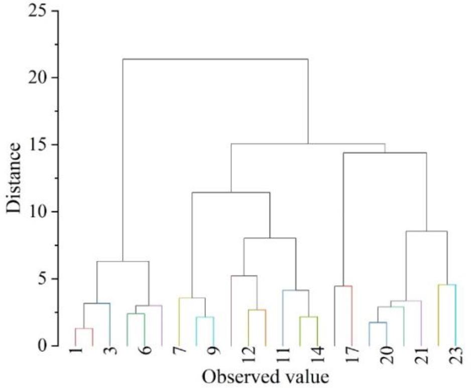
Group tree diagram of the community
In this paper, the following indicators are used to analyse the social network relatedness of the casual community members: the degree of relatedness, the degree of the hierarchy of the graph, and the nearest upper limit. UCINET 6.0 software was used to analyze the correlation between multiple-dimensional networks among members of the three groups, and the results of the analysis are shown in Table 7.
Social network correlation degree and hierarchy
| Index | Affective network | Information network | Consulting network | |
| First set | Connectedness | 1 | 1 | 1 |
| Hierarchy | 0 | 0 | 0.37 | |
| LUB | 1 | 1 | 0.92 | |
| Second group | Connectedness | 1 | 1 | 1 |
| Hierarchy | 0 | 0 | 0.28 | |
| LUB | 1 | 1 | 0.94 | |
| Third group | Connectedness | 0.78 | 1 | 1 |
| Hierarchy | 0.08 | 0.27 | 0.61 | |
| LUB | 1 | 0.97 | 0.71 | |
In the correlation index, only the third emotional network is 0.78, and the other correlations are all 1. This means that the social networks of the three groups of members are connected, except for the third emotional dimension, and there are individual members in the third emotional network who do not have connected paths, so these members cannot communicate with each other emotionally. From the graph’s hierarchy, all three groups of members’ counselling networks have different degrees of hierarchy, the third group has the most obvious hierarchy, with a hierarchy of 0.61, and the first and second groups’ counselling networks have a slightly weaker hierarchy. This suggests that there is asymmetrical accessibility between members in the counseling relationships of the participants in casual community activities, and that individual characters are more dominant in the counseling relationships. In addition, the emotional and informational networks of the third group also showed different degrees of hierarchy. This indicates that there is also asymmetry in the third group in terms of emotional and informational exchange, with individual characters dominating the network.In informal networks, LUB is the key to resolving differences or conflicts within the organization. The larger the value of LUB, the more individuals have people who can resolve the conflicts between the two; the smaller the value of LUB, the fewer individuals have people who can resolve the conflicts between the two, and the difficulty in resolving the conflicts will be increased. From the table, it can be seen that the LUB value of the third group of counselling network is relatively small, such that when there is a disagreement in the counselling exchange, it is relatively more difficult to resolve the conflict
In the process of community activities, a multi-dimensional relationship network has been formed among the participants, and the structure of each dimensional relationship between different members is also different. Through social network analysis, it has been found that there are a certain number of core members in each dimensional relationship, and there are active subgroups in the relationship network of the sparring community. At the same time, the activity level of each subgroup is related to the status and influence of its members. Analyzing the social relevance of the members of each group, it can be seen that the emotional network of the members of the third group is 0.78, and the relevance of the other groups is 1, which indicates that there is an asymmetry between the members in the relationship network and that the individual members occupy a dominant position and have a dominant nature.