Enhancing MRI diagnosis of myocarditis using deep learning and generative adversarial networks

Publicado en línea: 17 mar 2025
Recibido: 06 oct 2024
Aceptado: 03 feb 2025
DOI: https://doi.org/10.2478/amns-2025-0206
Palabras clave
© 2025 Haifeng Gui et al., published by Sciendo
This work is licensed under the Creative Commons Attribution 4.0 International License.
The clinical manifestations of myocarditis are diverse, and its etiology includes infection, autoimmune disease and drug toxicity, especially infection, which can develop into acute heart failure, cardiogenic shock and chronic dilated cardiomyopathy with the progression of the disease, and early definitive diagnosis is of great value to the treatment and prognosis [1-3]. With the gradual rejuvenation of the incidence of acute coronary syndromes, some of the clinical manifestations of myocarditis and auxiliary tests such as electrocardiogram and myocardial enzyme profile are extremely similar to those of acute coronary syndromes, and it is difficult to differentiate them by conventional tests [4-6]. Currently, endomyocardial biopsy is still considered to be the gold standard for the diagnosis of myocarditis, but due to its traumatic nature, high complication rate, and sampling error, it is less commonly used clinically [7-8]. Structural magnetic resonance imaging (MRI) can detect potential or pre-existing myocardial changes, and has the advantage of reproducible and noninvasive histologic evaluation in identifying myocardial edema, congestion, necrosis, and other myocardial injuries, which is of significant diagnostic value in patients with myocarditis [9-12]. However, due to their relatively low resolution and the presence of large layer spacing in the images, these diagnostic MRI data may mask early signs of myocarditis lesions, limiting the accurate assessment of small lesions and anatomical structures [13-15]. Many deep learning methods have demonstrated state-of-the-art performance in MRI super-resolution reconstruction tasks, which can be utilized to improve image resolution device-independently and relatively quickly [16-18]. This approach provides more potential resources for medical image analysis and research while improving image quality.
In this paper, we first explain myocarditis, MRI principle, deep learning, and generative adversarial network theory in detail, and formulate a generative adversarial network-based myocarditis MRI diagnostic model construction program. The MRI images of myocarditis provided by a hospital are used as the data source, and the initial data are preprocessed using Python tools, and the processed data are stored in the form of datasets and divided into dataset A (MRI-weighted images of the myocarditis dataset) and dataset B (MRI images of myocarditis), which provide data support for the subsequent research work. Aiming at the problem that traditional generative adversarial network data is difficult to train, we propose to use ResNet-34 network and U-Net network as generator and discriminator, and determine the loss function of both. The research experimental equipment is selected, the calculation principles of quantitative evaluation indexes (MAE, RMSE, PSNR, SSIM and PCC) are given, and the aforementioned research data sets are synthesized to simulate and analyze the loss function of the model and the application effect of the model, respectively, with the aim of enhancing the level and effect of MRI diagnosis of myocarditis.
Myocarditis is a kind of myocardial inflammatory disease triggered by infectious or non-infectious factors, such as myocardial cell degeneration, necrosis and fibrous tissue proliferation and other pathological changes, which can involve the endocardium and pericardium, and most often occurs in childhood, which is not conducive to the health of children [19-20]. The clinical manifestations of myocarditis are not specific, and it is difficult for children to accurately describe their own symptoms and feelings, so the diagnosis of myocarditis has always been a clinical challenge. Endomyocardial biopsy (EMB) is the “gold standard” for the diagnosis of myocarditis, but it is invasive and damaging to the body, and is especially difficult to be accepted by children’s families. At present, the diagnosis of myocarditis mainly depends on clinical symptoms and ECG, echocardiography, laboratory tests and other aspects of comprehensive judgment. Magnetic resonance imaging (MRI) has the advantages of high resolution, non-invasive, and can be examined many times, and has been used more frequently in the diagnosis of children’s heart diseases.
MRI is based on the principles of MR, which involves basic physical concepts such as the spin and magnetic moment of the atomic nucleus, the energy state of the spin magnetic moment in the external magnetic field, the conditions for generating nuclear magnetic resonance (NMR), and the action of the radiofrequency (RF) field on the magnetization intensity vector and the process of relaxation [21]. MRI involves three aspects, namely, excitation and measurement of the RF pulse train of MR signals, acquisition of the signal position by using the K-space coding and reconstruction of an image by using K space coding information to reconstruct the image in these three areas.
The changes of atomic nuclei under a strong magnetic field are shown in Fig. 1. When an MRI scan is performed on a patient, the hydrogen nuclei in the patient’s body are not only aligned in the direction of the main magnetic field, but also spin in an approximate frequency, but their phases in spinning are randomized, which produces a reticulated longitudinal magnetization in the direction of the main magnetic field.
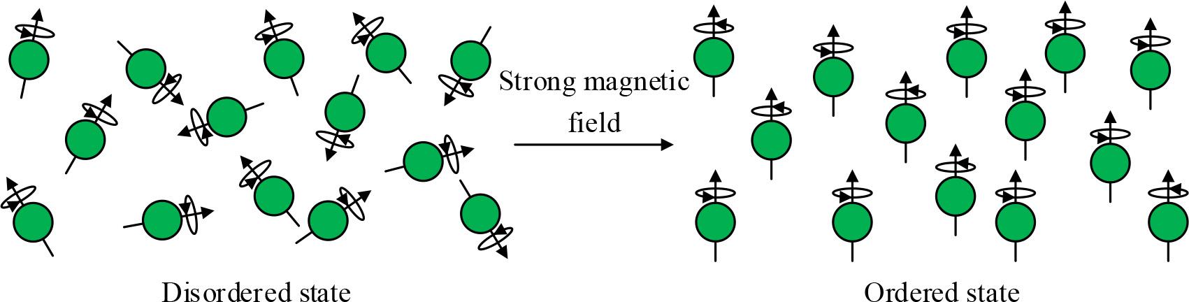
The change of atomic nuclei under a strong magnetic field
The change of the phase of atomic nuclei under RF pulse is shown in Fig. 2. Taking a tissue section as an example, the spinning in of all the hydrogen nuclei within the section is changed to the same phase under the RF pulse, and the nuclei are tilted to the x-y plane, and the longitudinal magnetization starts to decrease in this case, and a new transverse magnetization is gradually generated.

The phase change of the nucleus under RF pulse
The nuclei in the human body begin to return to their initial equilibrium state at the end of the RF pulse, and the pointing of the nuclei returns to the longitudinal direction again, a process known as relaxation. The relaxation process is divided into two types: the first is transverse relaxation, i.e., the transverse magnetization weakens and disappears at an exponential rate, and the time consumed by this process is called the constant T2; the second is longitudinal relaxation, i.e., the longitudinal magnetization returns to its original value at an exponential rate, and the time consumed by this process is called the constant T1. Remain constant, and the differences in relaxation times of different tissues form a fundamental element of MRI imaging. By varying the time between excitation of the nuclei and the time between excitation and the start of data collection, it is possible to control the emphasis of specific tissue features.
The rate at which the intensity component
The transverse magnetization strength
Transverse magnetization and longitudinal magnetization synthesize the total magnetic vector and move in a spiral motion with changing intensity and direction, the MRI spectrometer senses the current and begins to receive the signals emitted from the body, the current signal induced by the total magnetic vector gradually decreases and finally disappears but the frequency remains the same. The strongest signal is obtained after 90° pulse and the MRI image is reconstructed and the value of the signal received by the MRI spectrometer
The RF pulse sequence determines the contrast of the tissue signal; for long TRs (greater than 1500ms), the
The MRI operator can control the method of data collection and image reconstruction, for example, by changing the strength and rate of change of the auxiliary magnetic field, the pulse duration, and the sequence of data acquisition to change the artifactual effect of the image, the field of view, the contrast, the resolving power, and the speed of the acquisition, etc. The essence of these controls lies in the alteration of the K-space, which is fundamentally different from other imaging.
In myocarditis MRI, to better understand the imaging process, it is assumed that the heart area is partitioned into many small pieces, each of which is called a voxel. Assuming that a heart region is divided into sixteen voxels, the number of protons in each voxel is represented using shades of color, with lighter colors indicating a small number and darker colors indicating a large number, quantified as
In the actual measurement of hydrogen atoms, the measurements are derived from all the hydrogen atoms in the entire brain region. In order to obtain the number of hydrogen atoms in each voxel, a weighted integral about the concentration of hydrogen atoms is obtained by an additional gradient magnetic field:
The spatial variation of the magnetic field gradient demonstrates the inhomogeneity of the magnetic field and therefore allows the expression of each measured value:
Eq. (7) is a Fourier transform (4FFT) expression, while
Each point on the K-space is involved in the formation of the signal at all points on the MR image, so each point on the MR image does not correspond to each point within the K-space. In MRI, the middle of the K-space concentrates low-frequency information and has a decisive effect on the contrast of the MR image, while the edge of the K-space concentrates high-frequency information and has a decisive effect on the spatial resolution of the MR image. Therefore, the quality of MR images can be controlled by changing the K-space, which is fundamentally different from other images in terms of imaging principle, and by changing the K-space to control the image contrast, resolution and other characteristics.
Currently, MRI systems and CT systems in the field of medical imaging are very mature and are the main imaging modalities in modern medicine.MRI and CT have their own advantages and disadvantages, and to a certain extent, they can also complement each other. Table 1 shows a comparison of the performance of MRI and X-ray CT. The gray and white matter produced during MRI has a high contrast, resulting in a high quality cross-sectional image of the heart, which has led to a new stage in the diagnosis of conditions in the central nervous system.Table 2 shows the grayscales of normal human tissues on T1-weighted and T2-weighted.
Comparison of MRI and CT performance
| Imaging characteristics | CT | MRI |
|---|---|---|
| Imaging signal | X-ray | Radio-frequency energy |
| Imaging magnetic field | No | The superposition of static magnetic field and gradient magnetic field |
| Adopted electromagnetic wave | A narrow beam of X-rays | Radio-frequency wave |
| Fault direction | Generally perpendicular to the body | Arbitrary direction |
| Data acquisition mode | Multidirectional projection | Multidirectional or unidirectional projection |
| Imaging time for each layer | Ultra-high speed CT can reach about 10ms | It varies by scan sequence |
| Image reconstruction mode | Back projection method, convolutional back projection method, iterative method, etc | Two dimensional Fourier transform imaging is the main method |
| Ionizing radiation | There’s X-ray radiation | Very safe with very little RF radiation |
| Real-time imaging | Realize | Realize |
Gray scale of normal human tissue on T1 weighted and T2 weighted
| Name | 1 | 2 | 3 | 4 | 5 | 6 | 7 |
|---|---|---|---|---|---|---|---|
| T1 weighted | White grey | Black | Gray | White | Black | White | Black |
| T2 weighted | Gray | Black | White grey | Gray | White | White grey | Black |
To summarize, the advantages of MRI include (1) high soft tissue contrast without bone artifacts, (2) multiparametric imaging such as T1-weighted, T2-weighted, and PD-weighted, (3) multidirectional tomography including coronal, sagittal, and transverse planes, (4) cardiovascular blood flow imaging, (5) molecular level diagnosis, (6) good contrast enhancement with fewer reactions, and (7) high sensitivity to show lesions.
The shortcomings of MRI include (1) long imaging time, (2) motion artifacts, (3) insensitivity to show calcified foci, (4) specificity and accuracy of lesions are still not high, (5) more contraindications, and (6) high cost of examination.
Deep learning belongs to the machine learning technique, while machine learning belongs to the artificial intelligence research. The multilayer information nonlinear processing mechanism in the deep architecture of deep learning networks is used for pattern classification as well as other learning tasks, which emphasizes multilayer and nonlinearity. In fact, deep learning has its origins in artificial neural networks (ANN), which essentially refers to a class of methods for efficiently training neural networks with a deep structure. Deep learning is simply a neural network that includes many hidden layers, which first requires the construction of a deep machine learning model, and then use a large amount of data for training, followed by initialization, gradient optimization algorithms and other means to complete the learning and tuning of the network, and a reasonable model structure can learn the rich intrinsic abstract features that characterize the data, and establish a function mapping relationship from input to output, which will ultimately improve the classification accuracy. Using successfully trained network models, we can realize our requirements for automation of complex transaction processing. The basic models of deep learning neural networks are convolutional neural network (CNN), recurrent neural network (RNN), long short-term memory artificial neural network (LSTM), gated recurrent network (GRU), deep belief network (DBN), generative adversarial network (GAN), etc. For the study of MRI diagnosis of cardiomyositis, this paper mainly uses generative adversarial network (GAN).
A GAN consists of a generator G and a discriminator D, which are trained in competition with each other in the framework of adversarial training aimed at learning the probability distribution of real sample data [22]. The generator endeavors to generate fake data similar to the real samples by receiving input noisy data and learning to capture the latent distributions of the real data samples in order to confuse the discriminator’s inability to accurately discriminate the true from the false. Meanwhile, the discriminator works to do its best to determine the authenticity of the input data. Through mutual confrontation and optimization in the training process, the generator and the discriminator continuously improve their respective generating and discriminating abilities, gradually approaching the Nash equilibrium, in which the fake data generated by the generator can more realistically simulate the real data, while the discriminator can more accurately distinguish the real data from the fake data.
The network structure of GAN consists of two parts: generator network and discriminator network.
The generator is one of the core building blocks of GAN, which usually adopts the deep convolutional neural network architecture constructed by the upsampling layer and transposed convolutional layer to efficiently generate high-resolution sample outputs with spatially localized correlation. The input layer of the generator is directly fed with a random noise vector z, whose distribution is usually set to be Gaussian or uniform. Next are multiple fully connected hidden layers, each of which is connected to a ReLU activation function that progressively maps the noise to the feature space and extracts the abstract semantic information. Finally the output layer will add a Sigmoid activation function to map the hidden layer features to the target data distribution and output synthetic samples. The training objective of the generator is to maximize the probability that the deception adversarial discriminator considers the generated sample as a real sample. Through the confrontation process with the discriminator, the generator can gradually capture the distribution information of the training data and improve the realistic quality of the generated samples. Through the end-to-end multi-layer fully-connected network, the conversion mapping from simple random noise to complex real data distribution is realized, and high-quality synthetic data samples are generated.
In the GAN model, the discriminator and generator, whose role is to determine whether a sample is from a real data set, belongs to the binary classification problem. The structure of the discriminator uses a feed-forward multilayer neural network, the input is a real sample or a fake sample synthesized by the generator, and its output is a real-valued score, which is used to determine whether the input sample is from the real data distribution or the output of the generator. Specifically, the input of the discriminator first passes through multiple fully connected layers, and each hidden layer is followed by a ReLU activation function, which gradually extracts the features of the input sample. Finally, a sigmoid activation layer is connected, and the output of the discriminator is a real-valued score between 0 and 1, which indicates the probability that the discriminator considers the input sample belongs to the real data distribution. During training, the discriminator aims to output a high score close to 1 for real samples and a low score close to 0 for fake samples synthesized by the generator. By training against the generator, the discriminator is forced to continuously improve its discriminative ability to accurately distinguish the more realistic synthetic samples output by the generator.The adversarial relationship between G and D in GAN is shown in equation (8):
In the above equation (8):
The network structure of the basic GAN model is shown in Fig. 3. First, a set of random noise variables
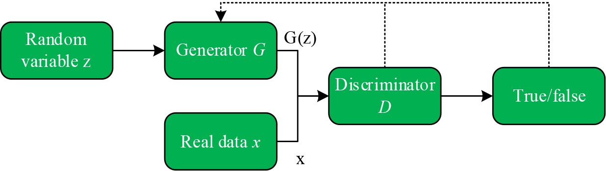
Network structure of basic GAN model
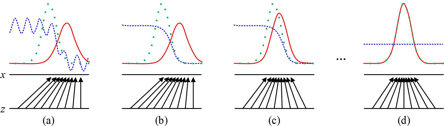
The training process of the Generative Adversarial Network (GAN) is shown in Figure 4.The training process of the GAN uses an alternating optimization approach where each iteration is divided into two phases. In the first phase, the discriminative model is fixed and the generative model is optimized so that the data it generates can be recognized as real as possible by the discriminative model. In Phase II, the generator is fixed and the discriminative model is optimized to improve its discriminative accuracy. Stages I and II are then looped and training is continuously performed, ultimately causing the generator to produce data similar to real data.
Generate a training process for adversarial networks (GAN)
In Fig. 4, x denotes the real sample data, z denotes the random noise vector input to the generator, the green dotted line denotes the real data distribution, the blue curve is the probability distribution of the discriminator’s discriminative output of the real and generated data, and the red solid line denotes the synthetic data distribution output by the generator. (a) The figure indicates that both the discriminator and generator are not trained to be randomly distributed, and at this time the discriminator cannot accurately determine whether the incoming data is real data or generated data. (b) The figure shows that after fixing the generator, the discriminator is trained and optimized, and the distribution of the output is close to 1 (true) in the interval of the “true” data distribution of the training set, and 0 (false) in the interval of the “false” data distribution generated by the generator, which means that the original data can be judged more accurately. That is, it is possible to more accurately determine the original real data or generated data after. (c) The figure shows that at this time the fixed discriminator, training generator, so that the output distribution of the generator converges to the distribution of real data. After the alternating training of steps (b), (c), (b), (c)…, it gradually makes the proximity of the data distribution of the generator’s output to the distribution of the real data smoother until it reaches the situation of figure (d), at this time, the green dotted line and the red solid line are completely overlapped, and the distribution of the generator’s output completely fits the distribution of the real data, which indicates that the generator learns the real normal distribution of the data.
The MRI diagnostic image of myocarditis is first acquired and preprocessing operations are performed on this image. On this basis, the performance of the network is improved by using the improved U-Net model as the generator of the GAN network and ResNet-34 as the discriminator. For the GAN network model, this chapter will mainly describe the algorithm flow and the improved GAN network structure.
The experimental data were provided by a hospital, and the data contained a total of 30 patients’ myocarditis MRI images, with about 180 sets of image data for one patient. One data set included one plain myocarditis MRI image without contrast injection and five enhanced myocarditis MRI images at five moments (moments 1-5) after injection of a conventional dose of contrast agent. The contrast agent used for injection imaging was gadopentetate dextran, with a contrast concentration of 0.1 mmol/kg, which was injected intravenously at an injection rate of 2 ml/s, followed by an injection of 50 ml of saline at the same rate in order to generate myocarditis-enhanced MRI images. When taking the enhanced MRI images, the 1-moment enhancement image was taken 30 seconds after injection of the contrast agent, and then every 90 seconds thereafter to obtain 5-moment enhancement images. The captured images had a size of 784 × 784 pixels, with a resolution of 0.45 mm corresponding to each pixel in the X- and Y-axis directions, and were divided into dataset A (MRI-weighted images of the myocarditis dataset) and dataset B (MRI images of myocarditis), to provide data support for subsequent research work.
The initial image format is DICOM format, first the image format is transformed to NII format file for saving using Python tool. The images were all 784×784 pixels in size and were cropped to 480×768 pixels in order to remove some of the black background area. Given that the data provided by the hospital in this experiment consisted of only 5400 sets of myocarditis MRI 2D images, the experimental data were expanded using data enhancement. The synthesized dynamic enhanced MRI images of myocarditis were then inverse normalized to obtain the data set form and stored.
In order to have better performance of the generator, U-Net network is used for the generator of the GAN network. The discriminator needs to judge the incoming real image and false image, due to the complex features of the two images, it is difficult to have good performance using a simple convolutional neural network, so the use of ResNet-34 network as the discriminator can deepen the depth of the network while improving its ability to extract features. In order to solve the problem of difficult to train GAN network, a BN layer is added between the convolutional layer and the activation function in both the generator and the discriminator. A detailed overview is given below:
The structure of the improved GAN network is shown in Fig. 5. Original Image denotes the image input to the generator, which in this chapter is the myocarditis MRI image at moment 0. Generator is the generator, which uses the improved U-Net network structure. Fake Image and Real Image denote the myocarditis-enhanced MRI image generated by the generator and the real myocarditis The Discriminator is a ResNet-34 structure that acts as a discriminator for the improved GAN network. The output result of the discriminator is calculated with the given label to calculate the binary cross entropy and then adjust the discriminator parameters by back propagation, BCE is the binary cross entropy in the figure. To train the generator, it is necessary to calculate MSE and GDL from the image generated by the generator and the real image, and input the generated image into the discriminator, get the predicted probability and then calculate BCE according to the label, and then use the weighted sum of MSE, GDL, and BCE as the loss function, and back-propagate in order to adjust the generator parameters.
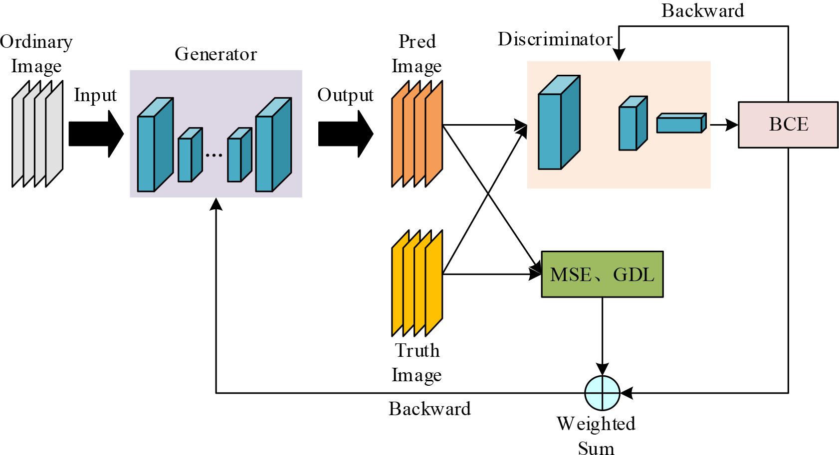
Improved GAN network structure
Myocarditis MRI image features are complex, the discriminator needs to extract more high-dimensional features in order to ensure its good performance, but at the same time, it also needs to consider the balance with the performance of the generator, so the discriminator adopts the structure of ResNet-34, which consists of a number of two-layer residual units stacked with two-layer residual unit structure.
U-Net is a deep learning network model. The network is similar to a traditional convolutional neural network, but there are differences.The U-Net network consists of four down-sampling blocks and four up-sampling blocks, each down-sampling block consists of two convolutional layers stacked with a pooling layer; each up-sampling block consists of two convolutional layers stacked with an inverse pooling layer, and finally, a dimensionality reduction operation is achieved by a 1×1 convolution to bring the network’s result output. Increasing the pooling layer can expand the receptive field, but the resolution of the lesion region in the MRI image of myocarditis is small, thus more features of the lesion region will be lost. In order to solve the above difficulties, the residual module is integrated in U-Net, which improves the problem of gradient vanishing while extracting more high-dimensional features.
In order to validate the effectiveness of the method proposed in this section and the enhancement performance of the network, this paper is trained and tested on the publicly available brain datasets IXI and MICCAI 2013 from different scanner models. In addition, tests using the public dataset of myocarditis, MRNet, are conducted to further validate the generalization ability of the network, and the MRI diagnostic model of myocarditis is augmented based on the generative adversarial network, where the generator consists of U-Net and the discriminator consists of ResNet-34, to validate the effectiveness of the model in this paper for practical applications through network comparisons. This subsection will give the detailed experimental design program, which contains the experimental dataset, sample preprocessing, experimental environment, and evaluation indexes.
In this section, three different datasets are used to evaluate the performance of the proposed model in this paper, including dataset A (MRI-weighted images from the myocarditis dataset) with dataset (MRI images of myocarditis) B. Dataset A was preprocessed to obtain 46,240 2D slices, and the data were divided into training, validation, and test sets according to the ratio of 3:1:1. Data set B contains 50 multimodal myocarditis MRI scans, and we used 2443 slices as the training set and 703 slices as the test set. Containing 1361 myocarditis MRI scans, we used 11,193 2D slices as the training set and randomly selected 3,500 slices as the test set.
The GAN method proposed in this section is implemented using the Python language based Pytorch framework and in a hardware environment with 11G Nvidia GeForce RTX 4080Ti GPUs. In the training phase, we optimize the network using the Adam optimizer and the dynamic learning rate with the initial value set to 0.0001, the batch size set to 25, and the training iteration period set to 500.To avoid overfitting and to improve the generalization ability, the model is optimized using a five-fold cross-validation. Specifically, the input dataset is randomly divided into five equal parts, with one part as the validation set and the remaining four parts as the training set each time, and the cycle is repeated five times, using a different validation set each time. This chapter evaluates the performance of the model on each validation set and takes the average value as the final result.
In this section, the reconstruction accuracy and quality of the proposed model is evaluated using the experimental evaluation metrics Peak Signal to Noise Ratio (PSNR), Structural Similarity Index (SSIM).PSNR is used as a measure of the reconstruction quality of an image, which shows the loss of detail in the reconstructed image.PSNR is defined as follows:
SSIM is a measure of similarity of brightness, contrast and structure between reconstructed image and real image, which measures the degree of similarity between two images.SSIM is defined as follows:
The regional mean square error (MSE) is commonly used to calculate the similarity between two target images, which is based on the overall degree of similarity between the two images, since the formula is calculated using the average of the overall differences. In this subsection, MSE and RMSE are used to measure the difference between the network-predicted myocarditis-enhanced MRI image and the real myocarditis-enhanced MRI image as the basis for adjusting the parameters of the network back propagation.MSE and RMSE are defined as shown in equation (11)(12):
In Eq. (11),
PCC denotes Pearle’s Selection Correlation Coefficient, and PCC can be calculated by the following formula:
The loss function is an important indicator of whether the parameter settings of the generative adversarial network are reasonable. The generative adversarial neural network generator and discriminator are composed of different functions: the generator is defined as
Most generative adversarial networks use the same discriminator loss function
The generator constantly input data, the discriminator constantly detects data, these two ends for repeated confrontation. The sum of generator and discriminator loss function is 0, i.e.:
For generator
The result of generator and discriminator loss function analysis is shown in Fig. 6, the output of the discriminator is expected to be as close as possible to 1 (judged to be real data), so the expectation is close to 1, and the training loss rate is 0 when log
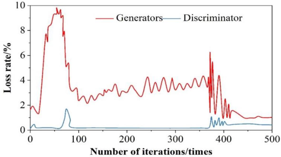
Analysis results of generator and discriminator loss function
Separate test set and training set put into the model of this paper for training, to get the results of the loss value of the test set and the training set, the results of the analysis of the loss rate of testing and training are shown in Figure 7. It can be seen that the loss rate of the generative adversarial neural network in training is 0. The test samples are put into the trained neural network for the training of MRI judgment of myocarditis, and through the continuous upgrading and evolution of the generator and discriminator, the fluctuation of the training compliance rate is getting smaller and smaller and decreasing, and ultimately approaching to 0 infinitely.
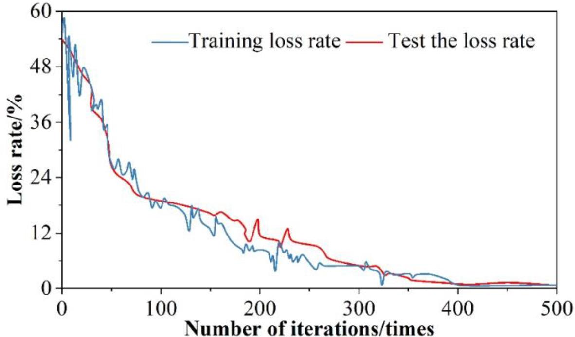
Test and training loss rate analysis results
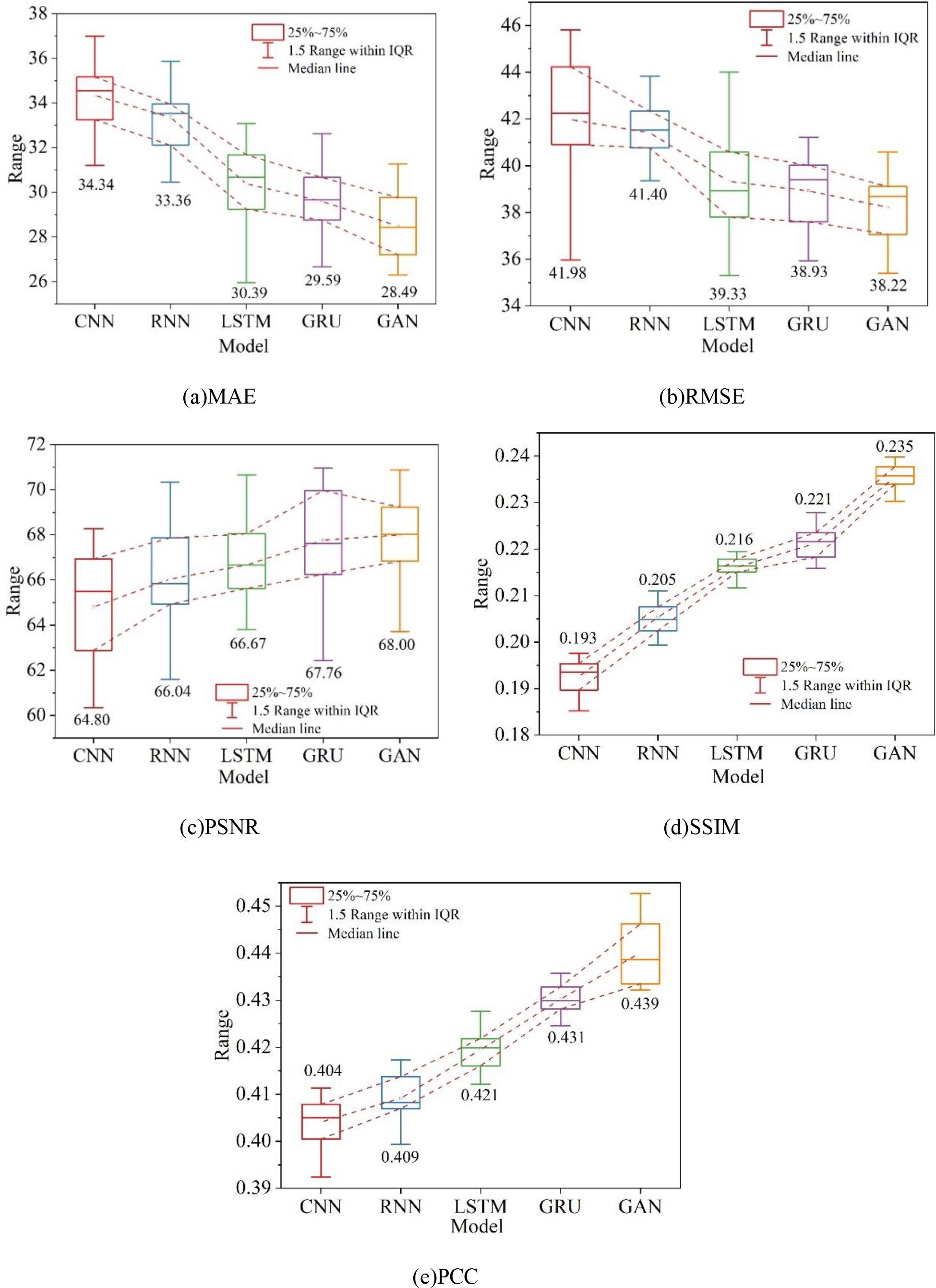
In order to verify the superiority of the two-branch adversarial network model, the experimental results are quantitatively compared with the representative medical image generation methods in recent years, which are CNN, RNN, LSTM, and GRU, respectively.For the five methods of the experiments, the average values of the data tests are given, and the overall five metrics (MAE, RMSE, PSNR, SSIM, and PCC) of the model quality are calculated. The experiments were all conducted under the same conditions, and the results of quantitative evaluation of different methods on dataset A are shown in Fig. 8, and the results of quantitative evaluation of different methods on dataset B are shown in Fig. 9, in which (a) to (e) are the MAE, RMSE, PSNR, SSIM, and PCC, respectively. The experimental results intuitively reflect the performance of CNNs and RNNs in enhancing the MRI images of myocarditis. The reason for this is that CNNs and RNNs are designed for general images and therefore have shortcomings in processing medical images. Overall the methods in this chapter perform better in terms of Mean Absolute Error (MAE) compared to the other methods, and all other evaluation metrics are also improved to different degrees. On dataset A and dataset B, the distribution of values of RMSE and SSIM metrics is slightly larger than that of GRU, and the stability needs to be strengthened, but the other metrics perform well. Comprehensive analysis of the proposed in this chapter based on generative adversarial network enhancement of myocarditis MRI diagnostic effect than other generative methods have been improved, and have reference value for the treatment of myocarditis.

Quantitative evaluation of results by different methods on dataset A
Quantitative evaluation of results by different methods on dataset B
Currently, there is a problem of unsatisfactory MRI diagnosis of myocarditis in hospitals, which is mainly due to the unclear MRI diagnostic image of myocarditis. In this regard, this paper proposes to enhance the MRI diagnostic model of myocarditis based on generative adversarial network, and evaluates the model of this paper from the two aspects of loss function and quantitative evaluation index.
1) When the number of iterations is 173, the generator loss function and discriminator loss function reach the maximum, with the increasing number of iterations, after 400 iterations of training, the loss of both are in a smooth state, and their loss values are 1.08% and 0.873%, which are within the tolerable range of the model. The test set and the training set are respectively put into the generative adversarial network, and it is found that after 400 iterations of training, the loss values of both are infinitely close to 0, which greatly ensures the effectiveness of the model.
2) In both dataset A (MRI-weighted images of myocarditis dataset) and dataset B (MRI images of myocarditis), the quantitative evaluation indexes (MAE, RMSE, PSNR, SSIM, and PCC) of this paper’s model are better than those of the other four models, which indicates that this paper’s model is of the highest priority for enhancing MRI diagnosis of myocarditis, and it fully verifies that this paper’s model has good practical application effect.