Lexical co-occurrence network and semantic relation mining based on English corpus

Published Online: Mar 17, 2025
Received: Oct 25, 2024
Accepted: Feb 09, 2025
DOI: https://doi.org/10.2478/amns-2025-0209
Keywords
© 2025 Guimei Pan, published by Sciendo
This work is licensed under the Creative Commons Attribution 4.0 International License.
According to the cognitive law of learning as categorization and the related research results of mental lexicon, vocabulary learning is the linkage of old and new knowledge, which includes the linkage of morphological, phonological and semantic relations between words. The vocabulary that people have learned is stored in the brain in the form of a network, rather than in alphabetical order as in a dictionary [1-4]. Among them, lexical semantic network is considered to be the most ideal model reflecting the organization of mental lexicon at present. In lexico-semantic networks, words are represented by nodes, which are connected to each other by morphological and phonological similarities and various semantic relations. The distance between the nodes is determined by the strength of the linkage between words [5-8]. Since vocabulary learning is not only about learning new words, but also about learning the relationships between words, the application of lexical semantic networks in learning dictionaries to provide the relationships between words will greatly benefit learners’ vocabulary acquisition [9-11].
With the in-depth development of semantically related lexical co-occurrence research, more and more language scholars have begun to pay attention to its application in university English vocabulary teaching. By analyzing the relationship between different words, semantically related lexical co-occurrence research can help students understand and memorize vocabulary better and improve their vocabulary use ability. Semantic lexical co-occurrence research can help students build vocabulary networks, promote vocabulary depth and breadth, and help students understand the real usage of vocabulary [12-15].
This paper analyzes the process of discovering semantic relations in the domain of English corpus using complex networks. The co-occurrence analysis method is proposed, the general process of the co-occurrence analysis method is elaborated, and the lexical co-occurrence relationship based on lexical semantics is summarized. Combining text complex networks and lexical co-occurrence networks, the TextRank algorithm is improved to optimize the extraction of keywords from lexical co-occurrence networks of text complex networks in the corpus. Combining the community discovery features of complex networks, the FWN-based short text clustering algorithm is proposed. Experiments are conducted to analyze the operational performance of the keyword extraction algorithm based on lexical co-occurrence network and the FWN short text clustering algorithm. Combine the sample corpus for lexical semantic analysis.
With the development of complex two networks, big data in network era provides rich data support for complex networks. And the research object of complex network is also beginning to be romantic to the real meaning, and its application field is also developed from a single mathematical graph theory knowledge application to the communication network, text network and so on. It makes it possible to simplify the complex real networks while realizing the structural characteristics of these networks from the internal exploration, and provides help for exploring the deep information of the actual network [16-17].
The basic properties of complex networks are as follows:
If there are
When calculating the node degree in a weighted network, in addition to the number of nodes adjacent to node
Where
The clustering coefficient is used to determine the degree of tight clustering of the nodes in a network, which reflects the local characteristics of different clusters in the network. If there are
where
Since complex networks are presented as graphs, the tight class coefficients can also be interpreted geometrically, if
For the above two characteristics, node strength usually measures the importance of individual nodes in the whole network. The concept of median is introduced to measure the centrality of a node in the global network, which is defined by the equation:
Where
The importance of nodes with large meshes is overly amplified in the calculation of the composite eigenvalue. For this reason, to address this hidden loyalty, the concept of centrality of meshes is introduced, which, in terms of meaning, is a normalization of the meshes of all nodes, which is calculated as:
Although there is no Euclid distance in complex networks, it can be replaced by the shortest path length, introducing the concept of centrality by proximity, reflecting the degree to which a node is at the center of the network, which Freeman defines as:
Where
The PageRank algorithm was first used in web page linking to determine the degree of influence a page has on the pages it links to. Its calculation formula is:
where
Up to now, the content characterized by the nodes in the text complex network model can be divided into words, phrases, sentences and paragraphs. As this paper in the construction of the network model also need to add the semantic information of words to maximize the retention of text information characteristics, so the selected text words as network nodes. The text network construction methods using words as nodes include three kinds of word-based co-occurrence, syntactic relationship-based and class-based dictionaries.
1) Text network model based on word co-occurrence
As the two necessary elements of complex network model are nodes and edges, nodes in the text network are composed of words, and the words can be obtained through textual disambiguation.
2) Text network model based on syntactic relations
3) Text network model based on class dictionary
Considering the connection between words in addition to neighboring co-occurring word relations. With syntactic relations, but also includes semantic relations between words. The calculation of semantic relationship is difficult to be realized by direct semantic calculation of words in the text, and the degree of similarity is usually measured by the semantic distance between words.
The calculation of semantic distance between words generally includes two ways based on domain knowledge and corpus.
In the process of complex network construction, the two most basic elements are nodes and edges. The most important thing in network construction for a certain complexity problem is that nodes and edges should be abstracted. The steps of discovering semantic relations in the domain of English corpus using complex networks are shown in Figure 1.
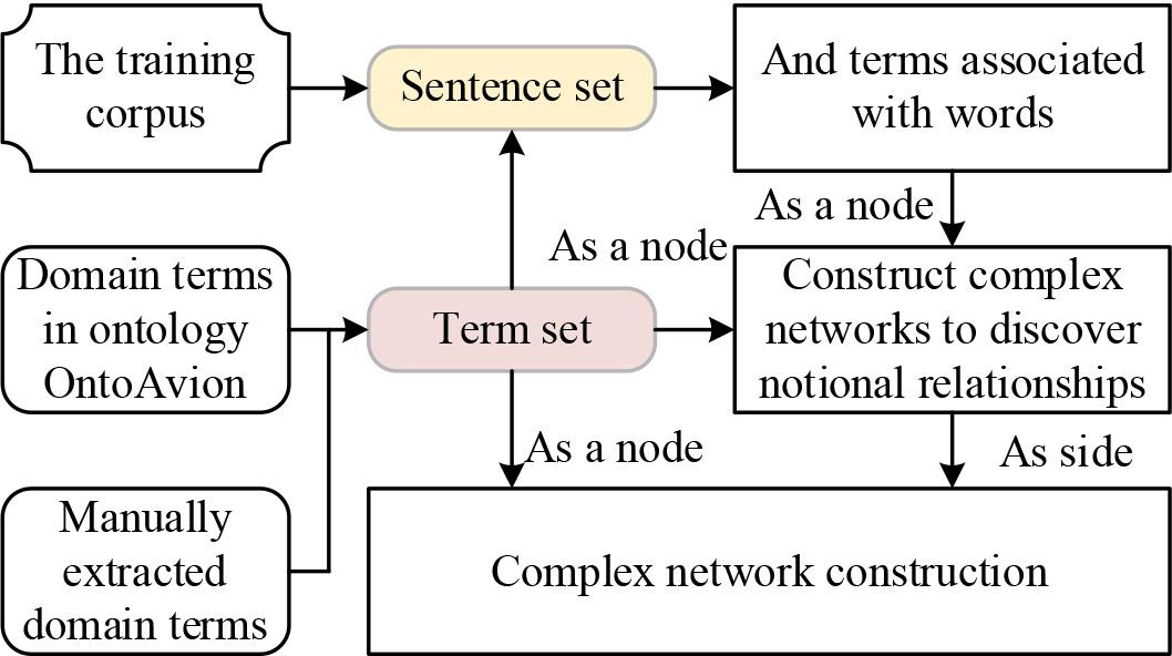
Complex network discovery semantic relationship steps
The relationship extraction process represented by the model can be briefly described by the following steps:
STEP1: Sentences are extracted from the training corpus to form the text set S of the sentences, this time using with the template method to discover the corpus used in the semantic relations.
STEP2: Analyze and get the concepts, objects within the domain by the terms and manual recognition in the domain ontology of the existing English corpus to form the term set T.
STEP3: According to the term set T, the words W associated with the terms, which can be verbs or nouns, are extracted from the sentence set S.
STEP4: The terms in the term set T and the extracted words W associated with the terms are used as nodes to construct the complex network. The formation of a community in the complex network represents that such terms have the same relation R.
STEP5: The complex network of the English corpus is constructed by using the term pairs in the term set T as nodes and the discovered relations R as edges.
From the semantic point of view of vocabulary, common lexical co-occurrence relations can be categorized as follows:
Oppositional relationship, where there is an oppositional relationship between two semantic constituents with the same table difference within the same semantic field between the semantic positions.
Overlapping relations-Relationships between semantic positions within the same semantic field.
Containment relation - When the semantic constituent of B is contained in the semantic position of A within the same semantic field, there is a containment relation between AB and AB.
Contextual relations-Relationships between semantic positions that are not part of the same semantic field. Comparable to contextual relations.
Relatively Irrelevant Relationships-Relationships that are not between semantic bits of the same semantic field. There is a relative irrelevance relation between two loci if their semantic elements do not contain each other.
Combinatorial relations-relationships that do not belong to the same semantic field.
A full understanding of the characteristics of lexical co-occurrence relations can play an important role in the effective utilization of these specific types of semantic relations that exist in the surface of language.
The general operation process of co-occurrence analysis is shown in Figure 2, which can summarize the general research process of co-occurrence analysis into three steps, data extraction, construction of co-occurrence matrix or co-occurrence vector, and data analysis. Due to the differences in the research objectives, the specific research process of co-occurrence analysis will also be different.
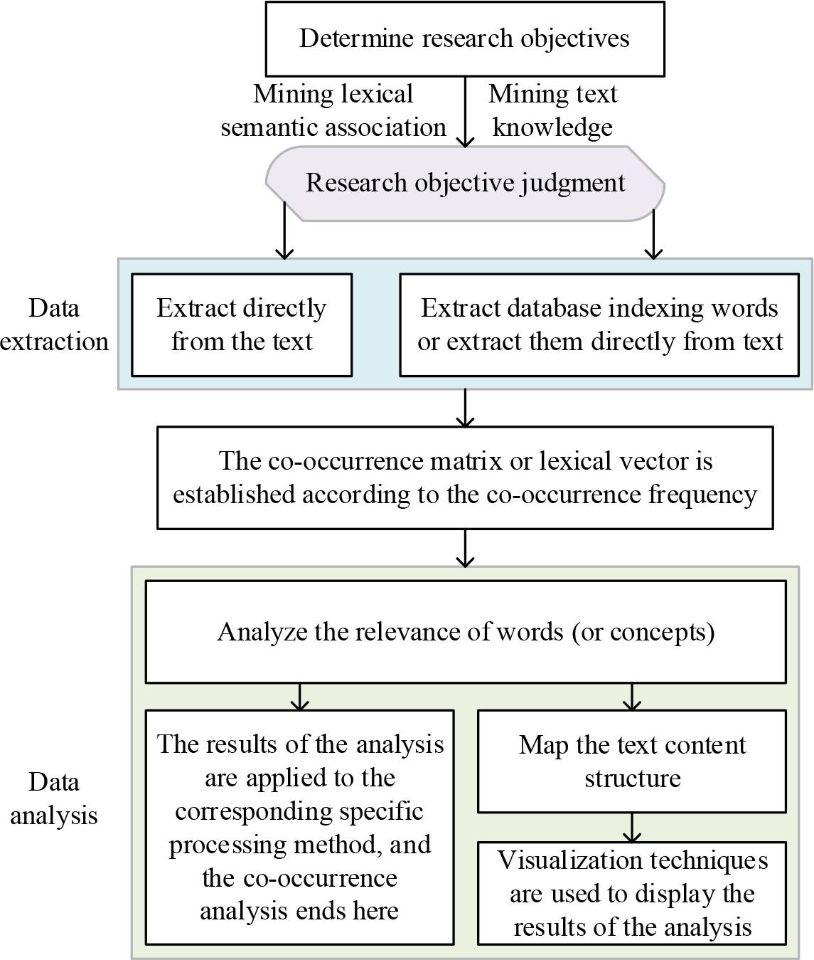
General operation process of common analysis
The collected co-occurrence information is analyzed using the lexical relevance approach. Relevance is a measure of correlation between objects characterized by dispersed attributes. Relevance quantifies the correlation between objects, which in turn clusters pairs of pairs with similar attributes into clusters. The relationships between words can be analyzed by calculating their relatedness, or words can be clustered to form concepts and the relatedness between concepts can be calculated. The main measures to process the first two types of co-occurrence matrices to analyze the correlation between words are Dice index, cosine index, and Jaccard index. The calculation formula is as follows:
where
The Jaccard index is widely used as a standardized correlation coefficient between two words representing
The correlation between two lexical vectors is usually calculated using the cosine index:
where
Sentence recognition is performed on the initial text T. The initial text T is divided into a collection of sentence
Word co-occurrence network
The steps of the improved keyword extraction algorithm for TextRank are specified as follows:
1) Construct word co-occurrence network. A series of preprocessing operations are performed on the text, and the word co-occurrence network is constructed on the basis of the word co-occurrence relationship of the processed document. 2) Initial node weight calculation. Considering the degree centrality and clustering coefficient value of each node in the network, the comprehensive feature value of each node is calculated and used as the initial weight of nodes in the network. 3) Connected edge weight calculation. The initial weight is assigned to the connecting edge between two nodes based on the importance of the node’s neighbors to it, so as to achieve the weighting of the connecting edge. 4) Keyword extraction. The C-TextRank algorithm is utilized for iterative calculation to obtain the importance ranking results of all nodes, and on the basis of which the node weights are updated by incorporating the node location features, and the top-K nodes are taken as the text keywords.
The algorithm is realized as follows:
When calculating the initial weights of nodes, this paper comprehensively considers the degree centrality and clustering coefficient of nodes in the computational text network two complex network statistical features.
The degree centrality
where
First, the comprehensive eigenvalue
Where
Where
In text, the position where the word appears is usually also an important factor in determining the importance of the word, and if the word
According to
The core idea of the FWN short text clustering algorithm is that there is a strong semantic connection between words that co-occur at high frequency. In order to better reveal the semantic connections between words, the FWN algorithm uses a complex network to model the topics in the short texts.The FWN algorithm treats words as vertices V in a graph, and there is an undirected edge E between two words if they occur together at high frequencies.It is shown that the network structure constructed in this way has the typical community structure where the words of the same topic are closely connected. structure. Therefore, by finding the communities of words that exist in the corpus word set co-occurrence network, we can find the feature word sets of topics that exist in the short texts. By utilizing the feature word sets of topics, short texts can be clustered.
Community is a common network structure often phenomenon appearing in complex networks, nodes with similar attributes are closely linked together presenting the structure of community, and nodes in different communities are relatively loosely connected to each other.
In this paper, the classical community discovery algorithm GN algorithm [18] is used in detecting the community structure present in the co-occurring network of English corpus.
Frequent itemsets refer to the set of data objects that co-occur at high frequencies. The frequency of the itemset refers to the number of data that have the objects of the thing and is called the support of the itemset. If the support of the itemset is greater than a predefined minimum support min value, the itemset is said to be called a frequent itemset.
FP-Growth frequent pattern growth algorithm is a classical frequent itemset mining algorithm. It uses the idea of partitioning to compress the set of data elements representing frequent itemsets into a frequent pattern tree called FP tree. This FP tree still retains the association data between these itemsets, and the FP tree algorithm treats the compressed data of things as conditional databases. Each database is associated with a frequent item, and for each conditional database only the data set associated with it needs to be considered.
A frequent word set is a set of frequent items of words in a large corpus, and a more rigorous definition of a frequent word set is given in Definition 1. Words in a frequent word set are used to represent the same set of concepts or to illustrate the same topic at a high frequency.
Let W be the short text data set
The short text clustering algorithm based on frequent word set word co-occurrence network, also called FWN short text clustering algorithm.The execution process of FWN short text clustering algorithm mainly consists of six steps as shown above and below:
1) Data preprocessing 2) Mining frequent word sets 3) Constructing FWN network FWN network, is a network constructed on the basis of word co-occurrence relationship of words in frequent word sets, i.e., all the words in a frequent word set are used as nodes. If two words occur in the same frequent word set then it is considered that there is an edge between these two words. In the FWN network constructed on the basis of frequent word sets, words within the same community, usually describe the same topic, i.e., the topic appears in the structure of a community. 4) Mining topic communities 5) Single-pole clustering After using the community discovery algorithm to find the topic communities that exist in the FWN network, the topics that exist in the corpus data and the set of feature words that these topics have are found. With these sets of feature words, one-poo clustering is performed by using a method that calculates the similarity between the set of feature words and the short text. Define the similarity between 6) Generate clustering labels After the above steps are executed, the FWN short text clustering algorithm accomplishes a typical text clustering task. That is, the input short text corpus data is automatically divided into multiple text clusters. The goal of generating class labels is to produce a readable and understandable label that provides a brief summary and description of the content of short texts within the same class of short text in-put.
1) The experimental environment includes:
Operating System: Windows 10 (64-bit)
Processor: Intel(R) Core(TM) i7 -1720HQ CPU 2.60GHz
Programming language: Java Matlab
Open platform: Eclipse 3.7 JDK2.5 Matlab 2023a
2) The experimental dataset of this paper adopts the condensed version of the Reduced Text Corpus, which is a corpus of English texts organized by a laboratory. The Reduced Text Corpus is derived from the news texts of an English news website, which mainly includes nine different categories of text datasets, such as sports, military, finance and economics, etc. Each category contains 2,000 different documents. Each category contains 2000 different documents, and the size of the compressed package is 60 M. Due to the fact that this dataset contains too much corpus, this paper will streamline and process the dataset in the following experiments, and select a part of it to be used for experimental simulation.
Based on the Reduced dataset, a total of 500 documents are extracted from 9 different categories and manually labeled with keywords, and a total of 2000 keywords are extracted. On average, 10.2 keywords are extracted from each document.
3) Experimental steps and parameter settings
The first step is to carry out the preprocessing of the text. It mainly includes Chinese word segmentation for each document, and this paper adopts FNLP word segmentation system. Then remove the deactivated words according to the deactivation word list and construct the candidate word set.
The second step of keyword extraction. The traditional TextRank algorithm and the improved algorithm are used for keyword extraction respectively, in which the specific experimental parameters are as shown in Table 1.
Since each document is manually labeled with 10.2 keywords on average, this experiment extracts the top 10 keywords for each document for comparative analysis. The number of sliding panes belongs to the uncertainty parameter, the experiment will be the number of panes were set to 2, 6, 10, 15, 20 to compare different experimental results.
4) Analysis of experimental results
For the experiment, the accuracy
The keyword extraction is performed according to the above procedure, and the keyword extraction results of the two algorithms at different sliding pane lengths are stored in the table. The comparison of the keyword extraction results is shown in Table 2.
The improved TextRank algorithm outperforms the traditional TextRank algorithm with the same sliding pane length. The results show that the optimization of edge weights of TextRank algorithm by combining the local semantic similarity of words is effective, which not only improves the accuracy of keyword extraction, but also reduces the time complexity and convergence of keyword extraction.
The results of the improved TextRank algorithm are better than those of the TextRank algorithm, with the average
Experimental parameter
| Parameter name | Parameter value |
|---|---|
| Maximum iteration number | 400 |
| Iteration out of the threshold | 0.003 |
| The single document extracts the number of keywords |
10 |
| Damping factor |
0.61 |
| Vertex score | 1.0 |
| Slide pane size |
2/6/10/15/20 |
Keyword extraction comparison
| Algorithm | Index | 2 | 6 | 10 | 15 | 20 | MEAN |
|---|---|---|---|---|---|---|---|
| TextRank | |||||||
| 0.3625 | 0.3212 | 0.3578 | 0.3755 | 0.3964 | 0.3627 | ||
| 0.4689 | 0.4968 | 0.4578 | 0.4772 | 0.4931 | 0.4788 | ||
| 0.3715 | 0.3251 | 0.3698 | 0.3745 | 0.3604 | 0.3603 | ||
| 53 | 56 | 59 | 52 | 51 | 54.2 | ||
| Improved textrank | |||||||
| 0.4596 | 0.4685 | 0.4725 | 0.4869 | 0.4911 | 0.4757 | ||
| 0.5521 | 0.5637 | 0.5417 | 0.5698 | 0.5927 | 0.5640 | ||
| 0.4122 | 0.4166 | 0.4867 | 0.4474 | 0.4516 | 0.4429 | ||
| 42 | 41 | 38 | 35 | 45 | 40.2 |
The dataset used in this chapter is from a corpus of English texts organized by a laboratory (ibid.). In order to verify the effectiveness of the short text clustering algorithm based on FWN, a total of 300 documents are extracted from 9 different categories, 1560 data are extracted number by number and the order of the text is disrupted, and then cluster analysis is carried out to obtain the clustering results. The number of texts in each dataset is shown in Table 3. The number of texts in the datasets of each category is different, and dataset 1 includes 526 text information.
Number of data sets
| Classification | Text quantity | Classification | Text quantity |
|---|---|---|---|
| Data set 1 | 526 | Data set 6 | 64 |
| Data set 2 | 125 | Data set 7 | 153 |
| Data set 3 | 348 | Data set 8 | 186 |
| Data set 4 | 56 | Data set 9 | 54 |
| Data set 5 | 48 | - | - |
In this paper, the results of short text clustering are judged using the check accuracy rate, check completeness rate and
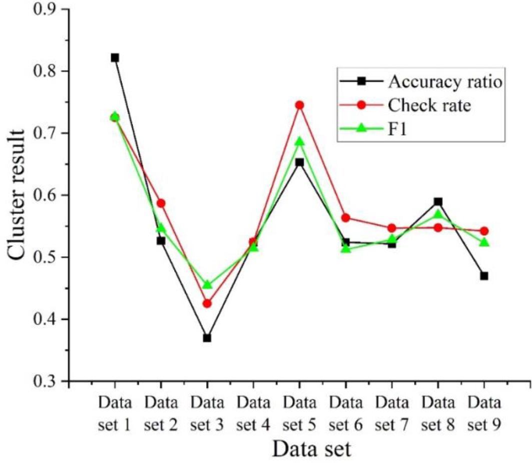
Clustering results evaluation
Wikipedia can serve different roles in different applications. In addition to being an encyclopedia, it is also considered a large-scale corpus, thesaurus, taxonomical map, conceptual hierarchy network, or ontological knowledge base. The different contents of Wikipedia sites contain a wealth of available resources, such as synonym page redirection, word disambiguation pages, structured infoboxes, hyperlinks to semantic web information, and taxonomical information classification maps. In this paper, Wikipedia is used as the research data.
In word co-occurrence network, each node represents a word and each word has a corresponding word class. By counting the nodes, the node characteristics of the network can be known. In the total network (which contains news domain word co-occurrence network, literature domain word co-occurrence network, and law domain word co-occurrence network), nouns have the highest number of nodes as nodes, followed by verbs. Time words have the least number of nodes as nodes. The order of the number of nodes from highest to lowest is: nouns > verbs > adjectives > adverbs > pronouns > temporal words > number words > exclamations > intonations > mimics > quantifiers > postpositions = connectives > modals > time words. The network nodes can then be better analyzed by comparing the three different domain words with the present network.
The distribution statistics of word categories of different domain word co-occurrence network nodes are shown in Figure 4. The three domains’ word co-occurrence network node word categories include nouns, adjectives, number words, quantifiers, pronouns, time words, adverbs, modals, mimics, postpositions, inflections, connectives, and exclamations. The largest number of nouns are distributed in the three domains of literature, journalism, and law, which include 8569, 7596, and 4021, respectively.
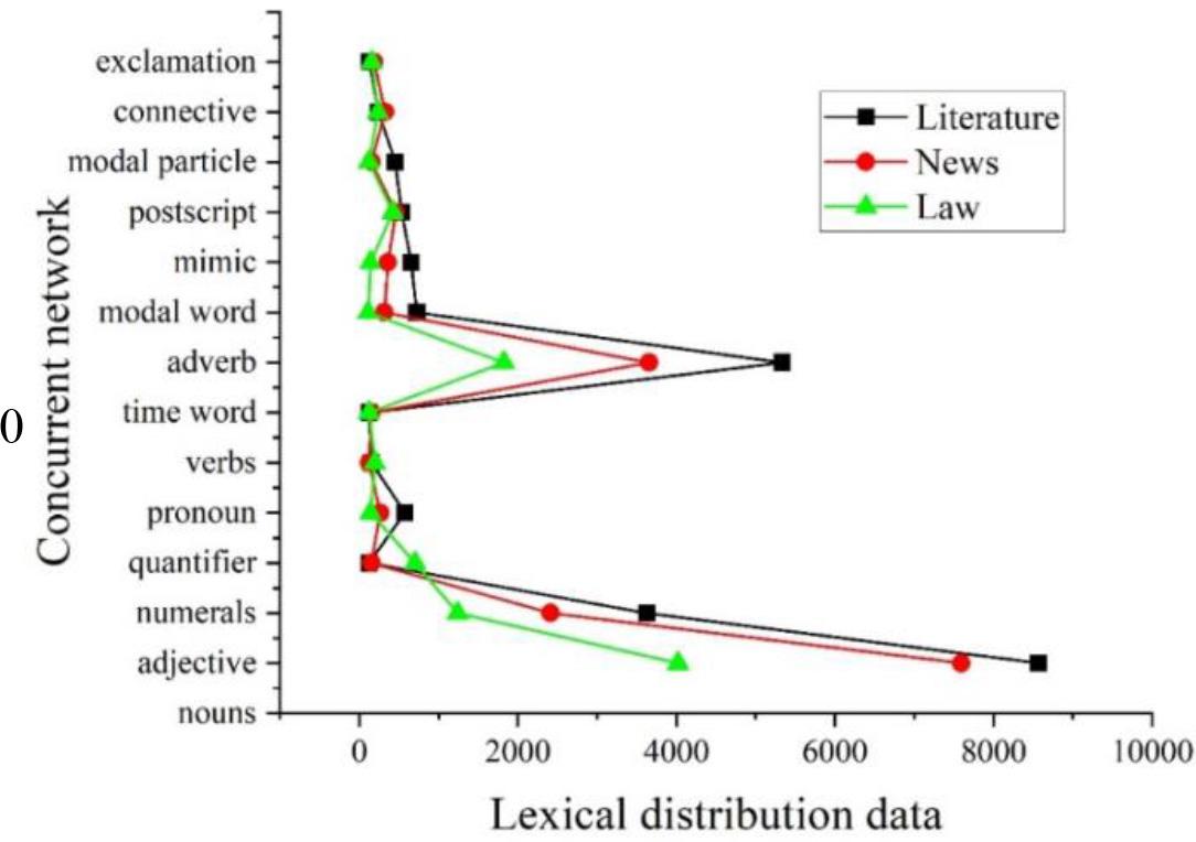
Different domain words and the node word distribution statistics
For the purpose of semantic relatedness evaluation, test sets have been created by manually annotating a collection of semantically related words. Certain publicly available test sets covering a larger number of keywords, which are widely cited in semantic similarity computations and experimental reviews. The Finkelstein-353 test set is a more typical manually labeled semantic similarity test set. It consists of a set of 153 word pairs covering 13 topics, and a set of 200 words covering 16 topics. The words are selected to cover as many possible semantic correlations as possible, and each pair of related words is manually labeled for semantic relatedness by 13-16 people. The average value is then selected as the final labeling result.
In order to review the multipath semantic relevance algorithm based on Wikipedia link graph, this test set is also used in this paper, using Wikipedia’s multi-language pairs of links, and also combined with a translation tool for translation and manual proofreading work on this test set, so that more words can be matched to nodes present in the English Wikipedia.
In order to evaluate the method of extracting semantically related words from the link references in this paper, and also to build a related word review dataset containing more vocabulary for the study of semantic similarity computation. The experiment manually labeled some of the semantically related words.
In order to ensure a certain degree of differentiation, the experiment did not completely select word pairs whose correlations are all particularly obvious. Instead, 800 word pairs from each of the two groups of words A and B were extracted from the set of semantically related words. Where group A are word pairs with high semantic relatedness. It was randomly selected from the set of words and from the set of words with average relevance in the range of 6-8. Group B is the word pairs with average similarity, which were randomly selected from the set of words with similarity in the range of 2-4. Further these related words were independently labeled with semantic relatedness by a team of 8 members and the results of their respective labeling were normalized. The average value was taken as the final result.
Some examples of the manual relevance labeling of the corpus are shown in Table 4. The table reflects the semantic relevance of the two terms, and the correlation between imperialism and colonialism, for example, is 0.472 for the two English terms.
Some examples of artificial relevance in corpus
| Word A | Word B | Degree of correlation |
|---|---|---|
| Imperialism | Colonialism | 0.472 |
| Shampoo | Conditioner | 0.399 |
| Overseas Chinese | Settlers | 0.085 |
| Lion tiger | Tiger lion | 0.551 |
| Yongding River | Lugou Bridge | 0.364 |
| First order logic | Field of theory | 0.261 |
| The middle ages | Castle | 0.277 |
| Symphony | Movement | 0.211 |
| Taiwan | NT | 0.316 |
| Husband’s family | Wife’s family | 0.387 |
| Hewlett-Packard | Printer | 0.428 |
| Spring Festival | Dumplings | 0.395 |
The experimental results of multipath semantic relevance calculation are shown in Table 5. Analyzing the experimental results, it can be seen that better results can be achieved by combining document graphs and classification graphs. And using any of the link diagrams alone may lead to worse results because of ignoring the useful semantic information. More desirable results can be achieved when the weighting factor of the classification diagram and document diagram is chosen to be
Multi-path semantic correlation calculation results
| Characteristics of the correlation algorithm | Grade correlation coefficient |
|---|---|
| Separate use of the classification diagram | 0.42 |
| Reciprocal path | 0.23 |
| Depth information weighting | 0.39 |
| Information content weighting | 0.37 |
| Use the document map separately | 0.36 |
| A non-directional diagram of a two-way link | 0.25 |
| Link to link separately | 0.37 |
| Link to the link | 0.31 |
| Forward to the connection and adjust the weight of the parameters | 0.41( |
| Use the first paragraph instead of English | 0.33 |
| Integrated document and classification diagram, and adjust the parameters | 0.46( |
| Open test masking(WS353) | 0.37 |
In this paper, we analyze the semantic relationship of text complex network, propose the co-occurrence analysis method, and improve TextRank algorithm for keyword extraction of lexical co-occurrence network. Combined with the lexical co-occurrence network in the English corpus for semantic relationship mining. The improved TextRank algorithm can reduce the time complexity and convergence of keyword extraction. In the comparison test, the results of the improved TextRank algorithm are better than the original algorithm, with the average
1) Project of Guangdong Provincial Private Education Association: Research on innovative application of College English Teaching in Private Universities under the background of digital transformation (No.: GMG2024084).
2) The Quality Engineering Project of Zhanjiang University of Science and Technology: Research on the optimization of online and offline resources and teaching practice under the guidance of innovation and entrepreneurship (No.: JG-2022546).