Numerical simulation and performance optimisation of in-cylinder friction of cylinder liner and piston ring in internal combustion engine based on deep neural network

Published Online: Mar 17, 2025
Received: Oct 11, 2024
Accepted: Jan 31, 2025
DOI: https://doi.org/10.2478/amns-2025-0164
Keywords
© 2025 Yichao Qian et al., published by Sciendo
This work is licensed under the Creative Commons Attribution 4.0 International License.
In today’s society, science and technology are developing rapidly. The requirements for mechanical products in the working environment are more and more demanding, the product structure is also more and more complex, and the user of mechanical products reliability requirements are increasing day by day. This means that the performance of mechanical products must be reliable. Users put forward higher requirements for the power source of mechanical products [1-3]. So far, as far as thermal efficiency is concerned, the internal combustion engine is deservedly the best among all power machines. Construction machinery, automobiles, ships, agricultural machinery, etc., without exception, will use the internal combustion engine as its power source [4-5]. Frictional wear is unavoidable in the working process of the internal combustion engine, and excessive wear will inevitably deteriorate the performance of the internal combustion engine, reduce the reliability of the whole mechanical product and even make the machinery prematurely obsolete [6-8].
Piston ring-cylinder liner friction is the largest sliding friction in the internal combustion engine. Internal combustion engines, especially diesel engines, large loads, unstable force state and other problems often lead to poor lubrication, which in turn increases the friction power loss of piston ring-cylinder liner [9-11]. The frictional wear problem is more serious during cold start. The lack of oil film and the wear of the cylinder liner and piston ring can also lead to a sharp increase in the amount of outgassing of the diesel engine [12-14]. The quality of the tribological design between the piston ring and cylinder liner is related to the power, reliability, fuel economy and emission cleanliness of the internal combustion engine, which in turn is related to the life of the internal combustion engine [15-17]. In recent years, people have mainly carried out the surface processing technology of piston ring-cylinder liner, tribological test design, reasonable selection of friction materials, optimization of lubrication state and other aspects of the analysis and research [18-20].
The first step in establishing the cylinder liner-piston coupling dynamics model is to analyze the dynamics of the cylinder liner-piston system.Key dynamic performance indicators, such as the trend of cylinder liner-piston ring friction in internal combustion engines, are obtained. Then, a multi-scale combined recurrent neural network model is proposed, which integrates the multi-scale feature extraction technique with the combined recurrent neural network (RNN) architecture and is equipped with the capability of nonlinear wear amount regression by capturing and learning the time-series features and their dynamic relationships during the cylinder liner wear process. In the experimental validation part, the article simulates and analyzes the piston ring, studies the influence of its structural parameters on the lubrication performance between the contact surface of the piston ring and the cylinder liner, designs the orthogonal test to optimize the piston ring profile, and analyzes the in-cylinder friction of the piston ring of the cylinder liner of the combustion engine before and after the optimization using the constructed prediction model for the wear on the cylinder liner surface of the internal combustion engine, in order to verify the validity of the optimization scheme.
The cylinder liner-piston system and forces are shown in 1, the motion model of the cylinder liner-piston system is shown in Fig. 1(a), and the force analysis of the piston is shown in Fig. 1(b).
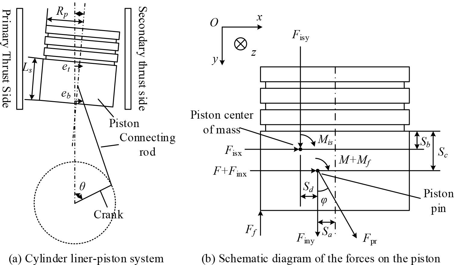
Cylinder liner - piston system and force
When the crank rotates at a constant angular velocity
Piston displacement:
Piston Speed:
Piston acceleration:
During the operation of an internal combustion engine, the piston not only makes reciprocating linear motion along the cylinder axis, but also accompanies the second-order motion, i.e., transverse swing, knocking the cylinder liner and rotation around the piston pin [21]. To analyze the force on the piston, the dynamic equations of the piston can be obtained from the force balance and moment balance as shown below:
Force balance equation for piston
Equilibrium equations for forces in the direction of piston
Moment balance equation for the center of the piston pin:
Where:
Set the top and bottom of the piston skirt transverse displacement were
Piston center of mass transverse motion displacement:
Displacement of the piston pin center of mass in transverse motion:
Piston swing angle:
Set the piston second-order motion acceleration of
Piston center of mass transverse motion acceleration:
Acceleration of transverse motion of piston pin center of mass:
Piston swing angle angular acceleration:
From Newton’s second law, the inertia force and moment of inertia acting on the center of mass of the piston as well as the center of mass of the piston pin are: transverse inertia force on the center of mass of the piston:
Piston pin center of mass transverse inertia force:
Piston center of mass longitudinal inertia force:
Piston pin center of mass longitudinal inertia force:
Piston center of mass moment of inertia:
Where
The second-order motion model of the piston can be obtained by substituting Eqs. (11)-(18) into the piston dynamics equations (4)-(6) and eliminating the connecting rod force
Where
During the operation of the internal combustion engine, the piston will produce a second-order motion, affected by the side thrust of the piston knocking the cylinder liner to produce a strong vibration. The vibration model of the cylinder liner and its force analysis are shown in Figure 2.
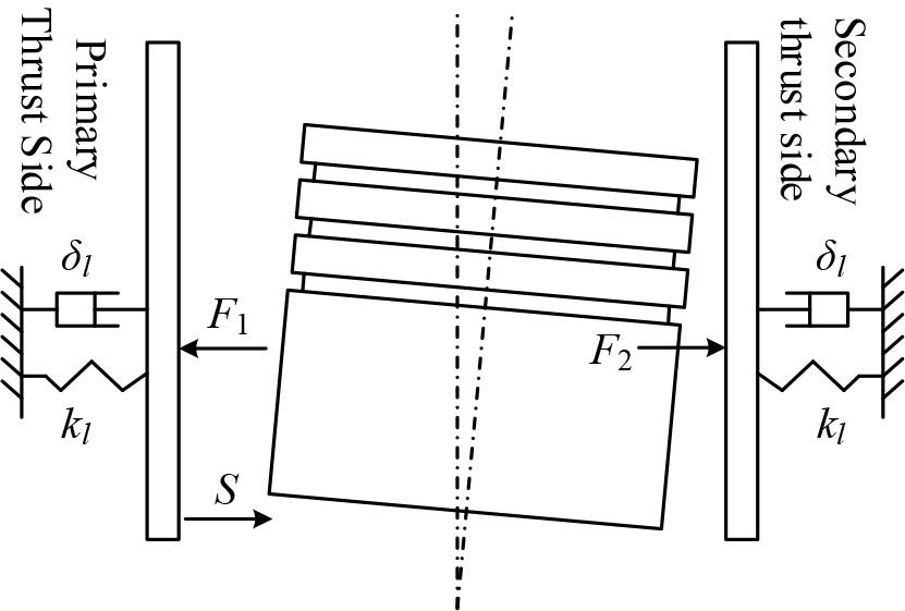
Jacket force
Let the mass of the cylinder liner be
The vibration response model of the cylinder liner considering the second-order motion of the piston can be obtained by coupling Eq. (19) with Eq. (22):
Internal combustion engine piston skirt and cylinder liner lubrication between the typical fluid dynamic pressure lubrication and oil film bearing area shown in Figure 3.
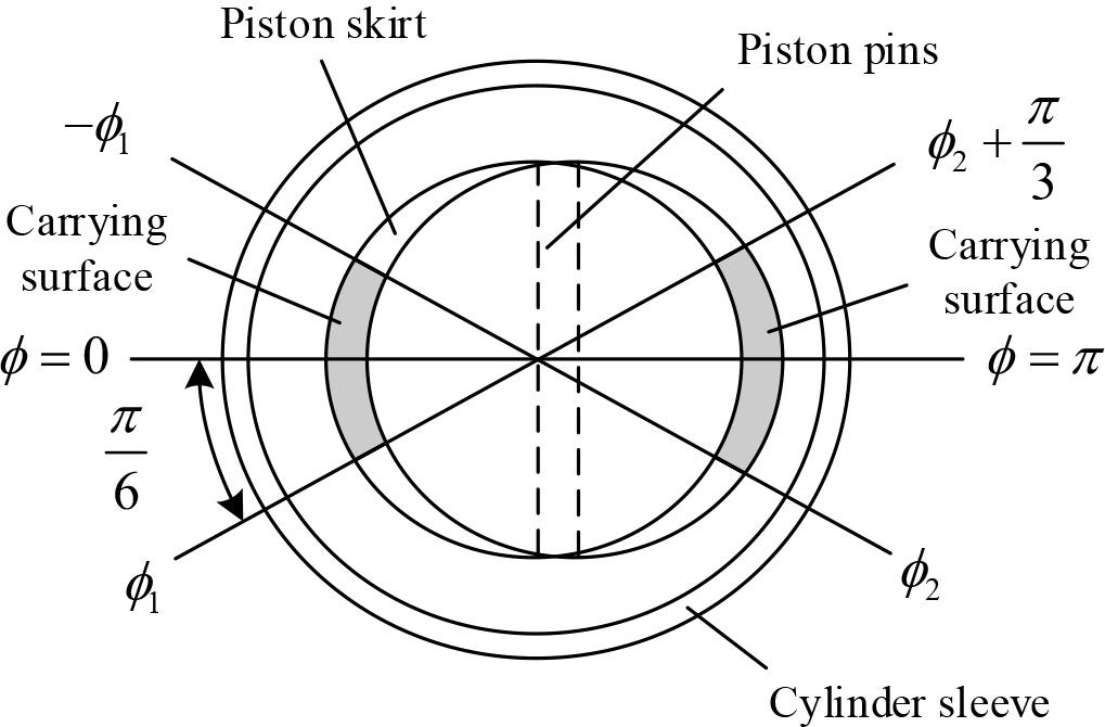
Oil film bearing area
For the cylinder liner-piston system, focusing on the lubrication between the piston skirt and the cylinder liner, the average Reynolds equation can be expressed as the cylinder liner is fixed to the body with a slip velocity of 0, and only the piston slides along the surface of the cylinder liner:
If the effect of piston and cylinder liner surface roughness on lubricant film stability is neglected, the oil film thickness between the cylinder liner-piston is the nominal oil film thickness
When analyzing the lubrication characteristics between the cylinder liner and piston, it is necessary to fully consider the lubricant film by the cylinder liner and piston surface roughness, in order to describe this effect, it is necessary to use the actual oil film oil film thickness
Where
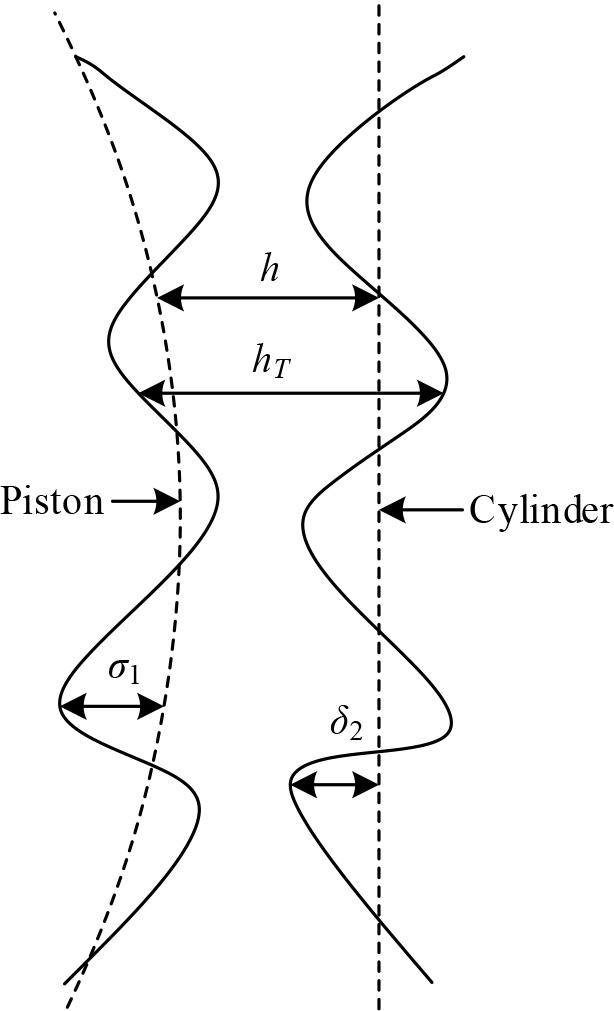
Lubricating oil film
Due to the complexity of the representation of the actual oil film thickness, which makes the analysis process very cumbersome, in order to simplify the analysis process, the concept of the average value of the actual oil film thickness
where
Thus, the right end of the Reynolds equation can be written as:
Introducing the dimensionless contact factor
The oil film pressure boundary conditions are as follows:
At the upper boundary
The oil film pressure acts only in the oil film carrying area, outside the carrying area the oil film pressure is zero:
Considering the symmetry of the piston skirt, when calculating the oil film pressure, only half of its area (0≤
By solving the average Reynolds equation, the distribution of the oil film pressure
In analyzing the effect of cylinder liner-piston skirt surface roughness on the lubricant film, the shear stress induced by the action of fluid dynamic pressure can be expressed as:
Where
The friction force acting on the piston skirt produced by the action of the dynamic pressure of the lubricant and the resulting friction moment is calculated as:
The micro convex body contact model proposed by Greenwood and Tripp is used to calculate the contact pressure generated by the contact between the two, which is expressed as:
Where E is the integrated modulus of elasticity,
Where
Solving the above equation yields:
Simplified and obtained:
At the cylinder liner and piston skirt microscopic level, when solid-solid contact occurs between the two, the shear stress generated by the interaction between the cylinder liner and piston skirt micro convex body surface is:
Where
After finding the friction force, the friction power consumption of the cylinder liner-piston system can be found according to the mechanical power calculation formula:
In this paper, it is assumed that the height distribution of the micro-convex body on the inner wall surface of the piston skirt as well as the cylinder liner obeys the Gaussian distribution, and according to the characteristics of the Gaussian distribution, the calculation of each factor is based on its numerical fitting formula.
Calculation of flow factor
According to the literature, the fitting formula of the pressure flow factor is:
Contact factor calculation
The literature gives expressions for the contact factor for the four commonly used distribution types, and the contact factor fitting equation for the Gaussian distribution of the height of the microconvex body is:
Shear stress factor:
In this study, 1 model is proposed for predicting the amount of wear on the cylinder liner surface of an internal combustion engine. The input information to the model is the cylinder liner wear over time per unit time, which is used as the input to the main body of the network after min-max normalization for scaling the data interval. The main part of the network adopts a combined structure of 2-layer serial LSTM and 2-layer parallel GRU, in which the number of the three hidden layers is in the ratio of 1:2:4. The 2-layer LSTM at the front end extracts temporal features and long-term dependencies from the forward and backward directions, respectively, to provide comprehensive temporal information for the model, and the parallel GRU at the back end further deepens the model’s learning of complex features and relationships.
In order to preserve the original information, residual connectivity is used for both internal and head-to-tail features of the network. The residual connection enables cross-layer transfer of features by introducing jump connections between layers, which helps to alleviate the gradient vanishing problem and improve training efficiency.Finally, data prediction is performed using fully connected layers and regression layers. This design enables the model to learn the input sequence in an end-to-end form and predict the wear on the cylinder liner surface [23].
Min-max normalization is 1 common method of data interval scaling, which transforms the value domain of the input data into a fixed interval:
Where:
LSTM controls the flow of information by introducing a gating mechanism to effectively capture and memorize the long-term dependencies in a sequence. The basic unit of the long short-term memory network is shown in Fig. 5. The input state is
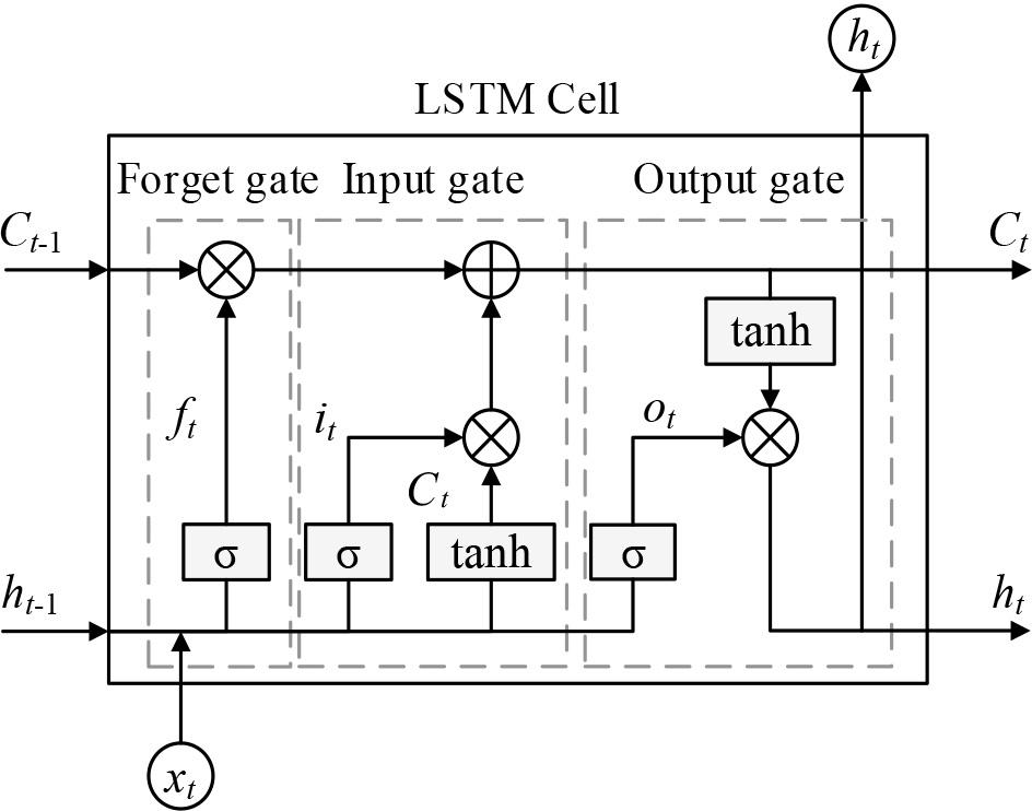
Basic units of long short tcrmmemory netw orks
The input gate is responsible for filtering the amount of information received: the input data and previously hidden states are processed through a Sigmoid activation function, which outputs a value between 0 and 1 to determine the amount of information allowed to pass through, the mathematical expression for the input gate is
Where:
The forgetting gate is used to determine the amount of information discarded in the cell state. It employs a Sigmoid activation function, which determines the extent to which previous cell states are discarded. The mathematical representation of the forgetting gate is
Where:
The cell update state step remembers or ignores the current input. Using the tan
Where:
The formula for cell state update is expressed as
Where:
The output gate determines which part of the cell state will be output based on the current input and hidden state, which uses the Sigmoid activation function and the tanh activation function, denoted by Eq:
Where:
The final hidden state and passes through the output gate
The bi-directional LSTM layer is based on LSTM, where past and future information is considered at each time step in chronological order and reverse chronological order, respectively. The hidden information states are connected to provide a more comprehensive contextual understanding through the flow of information in the 2 directions. It has a more powerful inverse evaluation capability to utilize past and future information to make more reliable model predictions. Its integrated hidden state is represented as:
Where:
The bidirectional LSTM layer learns the features of the input sequence more comprehensively than the two-layer stacked LSTM layer, which helps to save the design cost of the subsequent model architecture and reduce the number of parameters.
Gated Recurrent Unit (GRU) is another RNN variant for processing sequential data. Similar to LSTM, GRU is designed to simplify the structure of LSTM by introducing update gates and reset gates while still being able to efficiently capture long-term dependencies.
The synthesized hidden state of the bidirectional LSTM is used as the input state of the GRU, denoted as:
Updates the computation of gate vector
Where:
Computation of the reset gate vector
Computation of new candidate hidden states:
Updates the calculation of the hidden state:
In this paper, we design a 1 multi-scale feature extraction architecture based on GRU units, and the number of bi-directional LSTM and GRU hidden layers set up in the paper are 100, 200 and 400, respectively, with the ratio of 1:2:4, which indicates that for each bi-directional LSTM layer, there are 2 GRU layers of different scales in parallel. For GRU layers operating on different scales
Where:
Each of the different scale layers outputs 1 feature vector that encapsulates the information learned at a particular scale, and then the feature vectors are fused by a form of cascade operation:
The multi-scale structure enables the extraction of features at different levels of abstraction. Bidirectional LSTM layers capture patterns in the data that are more detailed and smaller in granularity. The GRU layers are larger and focus on broader trends, and this hierarchical feature extraction is key to predicting the progression of wear dynamics.
Bidirectional LSTM units are good at understanding long-term dependencies but can be computationally expensive. By having a smaller number of bi-directional LSTM units, it can be ensured that these units focus on capturing the most important long-term trends. In contrast, GRUs efficiently process data at a higher temporal resolution, capturing short-term correlations that are also critical for accurate prediction. In contrast, a larger number of GRU units can increase network capacity without causing any complexity. Thus, increasing the number of GRU units by a factor of 1 can provide the network with more functionality for complex modeling without making training too difficult. The structure of the multiscale temporal network is shown in Figure 6.
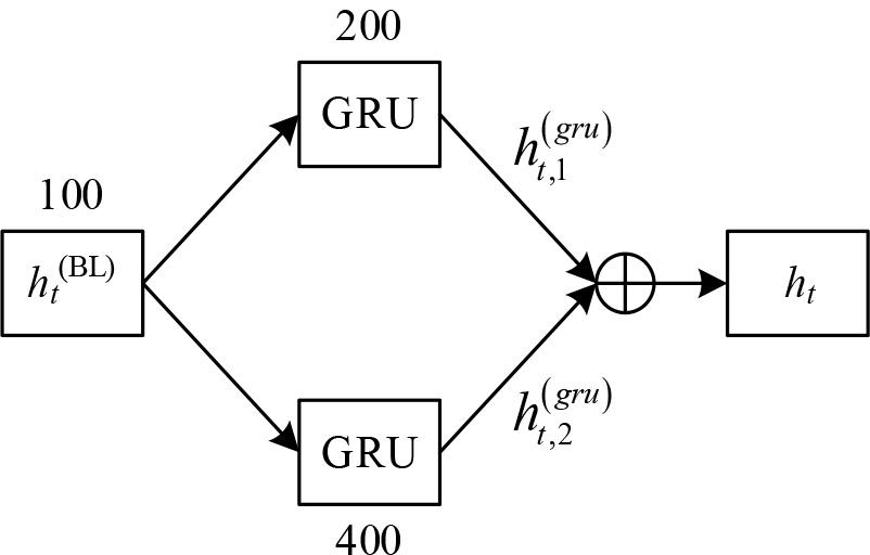
Multi-scale temporal network structure
In order to facilitate the direct propagation of gradients and thus alleviate the gradient magnitude decay often encountered in deeper network training, in this paper, pathways are established between multiple modules by means of residual connections, which enhances the ability of the network to be trained efficiently at a deeper level. The residual connections of the forward and reverse LSTM are denoted as:
The residual connection between GRU and the original input data is denoted as:
Residual layer connectivity refines the feature representation propagated by the previous layers, thus preserving critical information in the depth of the network and enabling feature extraction to be enhanced without degrading the accuracy of the characterization.
This section of the experiment focuses on the impact of the coupled analytical model of piston second-order motion-cylinder liner vibration response and the fluid dynamic-pressure hybrid lubrication model established in this paper on the numerical simulation of friction and performance optimization of the friction in the cylinder liner-piston ring cylinder of an internal combustion engine.
The variation of oil film thickness with crankshaft rotation angle at different barrel heights is shown in Fig. 7. The relationship between the oil film thickness between the two lubricating surfaces of the piston ring and the cylinder liner varies with the crankshaft rotation angle. According to the image, it can be seen that the peak of the oil film thickness appears near the upper and lower stops of the piston stroke, which is because when the piston moves to the vicinity of the upper and lower stops, its running speed is the smallest, and due to the stroke process of scraping the oil, at this time, the lubricating oil between the surface of the piston ring and the surface of the cylinder liner has a large amount of agglomeration, and therefore the oil film thickness near the upper and lower stops is larger. When the upper and lower stops are reached, the piston speed becomes 0. At the instant of reverse motion, the oil film thickness decreases sharply, even to 0. After the start of reverse motion, the thickness of the oil film increases due to the scraping of oil by the piston ring. When the height of the barrel surface is 1.5μm, the thickness of the oil film is obviously smaller than the thickness of the oil film when the height of the barrel surface is 4μm, but with the increase of the barrel surface height, the thickness of the oil film is not getting bigger and bigger, and when the height of the barrel surface is increased to 12μm, the thickness of the oil film is smaller than the thickness of the oil film when the height of the barrel surface is 8μm. This is because the extrusion effect of the piston ring mainly determines the size of the oil film thickness. Too large and too small barrel heights are not conducive to the formation of the extrusion effect of the piston ring, so the barrel height should be more reasonable.
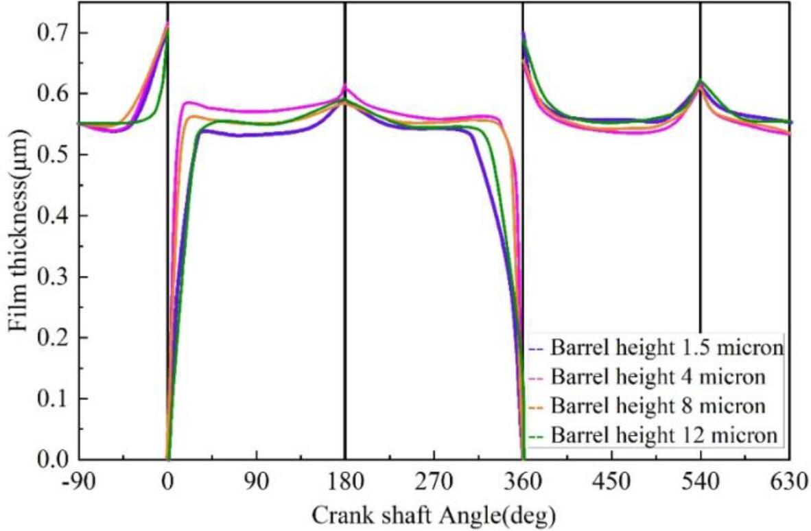
The thickness of the oil membrane under different barrels is changed
The influence of the barrel surface height of the piston ring on the friction force and friction loss of the piston ring-cylinder liner friction pair is shown in Figures 8 and 9. When the piston ring moves near the upper and lower stops, its speed is very low. At this time, the micro-convex body friction is the main force between the piston ring and the cylinder liner, and the larger the barrel surface height of the piston ring, the larger the micro-convex body friction is. In the process of piston movement, fluid friction is the main force between the piston ring and cylinder liner, and the thickness of oil film produced by smaller barrel height is larger, so the fluid friction is also larger. In the whole movement process, fluid friction accounts for the main part. When the barrel height of the piston ring is larger, the total friction between the piston ring and cylinder liner is smaller, and the total friction loss is also smaller, so the friction and friction loss between the piston ring and cylinder liner at the barrel height of 8 μm is smaller than that of the friction loss at the barrel height of 1.5 μm and 4 μm. However, when the barrel height is too large, the relative area between the piston ring and the cylinder liner decreases, resulting in increased friction loss throughout the stroke, and the friction force and friction loss between the piston ring and the cylinder liner increase to different degrees when the barrel height is 12μm.
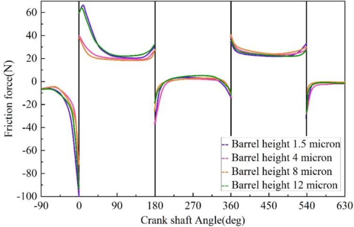
The friction of the different barrels is changed with the crank shaft
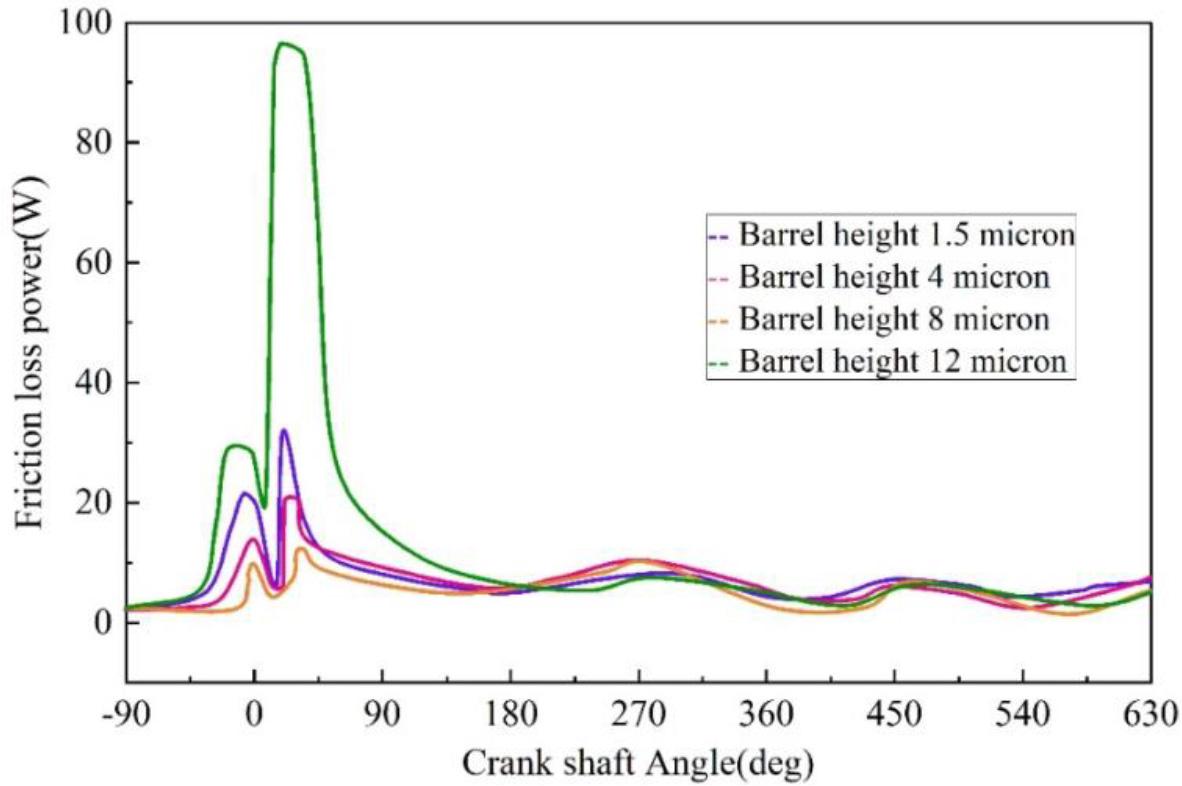
The friction loss power of different bucket levels varies
Depending on the actual situation, barrel-faced piston rings do not always take the form of a symmetrical barrel face, and the highest point of the barrel face the highest point of the barrel face is sometimes shifted toward the combustion chamber or the second gas ring, which is called barrel face offset. The highest point of the barrel face is moved towards the combustion chamber or the second gas ring.
The offset of the highest point of the barrel face toward the combustion chamber is called the positive barrel face offset, and the offset towards the second gas ring is called the negative barrel face offset.The variation of oil film thickness, friction, and friction loss power between the piston ring and cylinder liner with different barrel surface offsets as a function of the engine crankshaft angle is shown in Fig. 10, Fig. 11 and Fig. 12. From the figure, it can be seen that in the upward process of the piston, the oil film thickness of the piston ring barrel surface negative offset is slightly larger than the barrel surface positive offset and barrel surface symmetrical piston ring oil film thickness, while in the downward process of the piston, the oil film thickness of the barrel surface negative offset is relatively small, the oil film thickness of the barrel surface positive offset is the largest, and the oil film thickness of the larger barrel surface positive offset to be relatively large. For example, when the crankshaft rotation angle of 90 °, the barrel surface offset 30 μm, the oil film thickness of 0.52 μm, the barrel surface offset 60 μm, and the oil film thickness of 0.5 μm. Barrel surface positive offset friction and friction loss are smaller than the barrel surface negative offset and the barrel surface of the nominal piston ring. This is because, during the upward movement of the piston, the barrel faces a negative offset piston ring, and the wedge gap between the end face of the piston ring and the cylinder liner is more favorable to the formation of the lubricant film. In contrast, when the piston ring moves downward, the result is just the opposite.The barrel faces a positive offset of the oil film thickness, which is relatively the largest. The more barrels face positive offset, the longer the wedge inlet formed by the piston ring and the cylinder liner wall, the more conducive to the formation of the oil film, and therefore, the larger the barrel faces positive offset. Therefore, the oil film thickness formed by the larger barrel positive offset is larger. Overall, the positive offset of the barrel surface can effectively reduce the friction force and friction loss, so that the moving parts are in an ideal lubrication state.
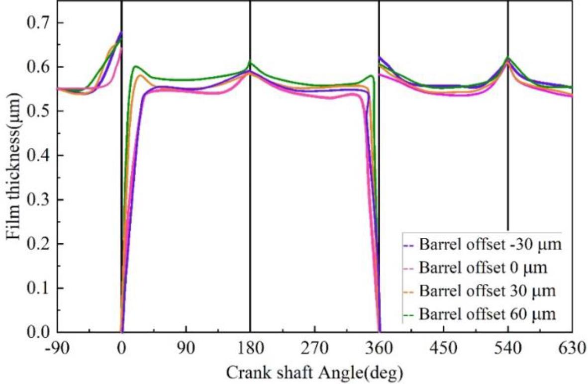
The thickness of the oil film varies with the crank shaft
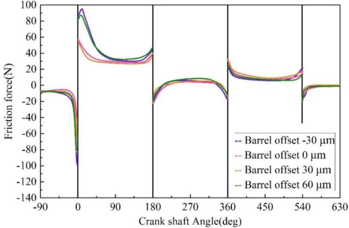
The friction of the crankshaft is changed by the friction of the crankshaft
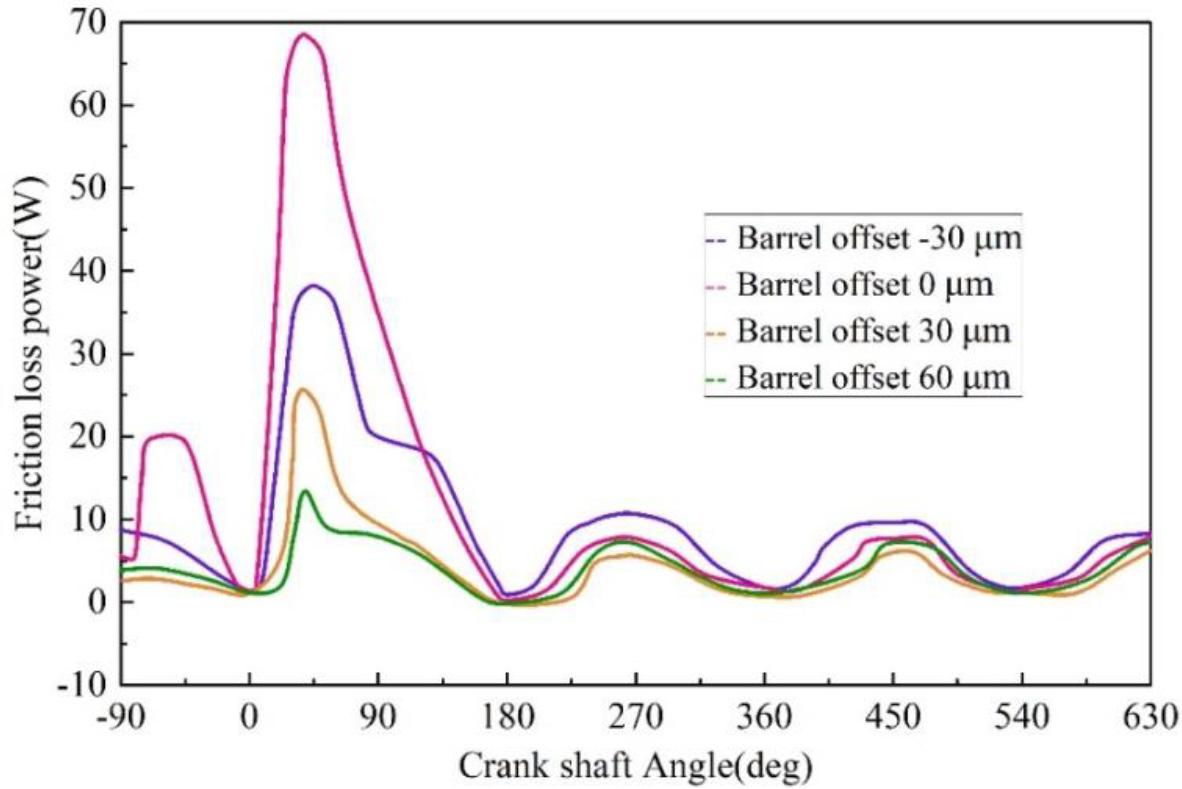
The friction loss power is related to the change of the crankshaft Angle
Due to the piston ring installation process needs, a certain closed gap, closed gap for the piston installed to the piston ring groove and is in the working state of the piston ring between the distance between the cut end face. Due to the existence of the closed gap, the piston ring is allowed to have a certain expansion and contraction margin when the piston is working, which can effectively reduce the piston ring stuck in the piston, and reduce the seriousness of the piston ring will cause cylinder pulling, melting or even broken, so the piston ring closed gap plays a very critical role in the smooth operation of the piston. This paper establishes the closing gap for the piston ring in the cold state.When the engine is working, the piston ring expands at high temperatures, and the closing gap in the hot state is smaller than the setting value in the cold state.The relationship between oil film thickness, friction force, and friction loss power with crankshaft angle at different closing gaps is shown in Fig. 13, Fig. 14 and Fig. 15. The variation of oil film thickness, friction force and friction loss power between piston ring and cylinder liner with crankshaft rotation angle under different closing clearances are shown in Fig. 13, Fig. 14 and Fig. 15, respectively. From the figure, it can be seen that the oil film thickness between the piston ring and the cylinder liner is gradually smaller with the increase of the closure gap and decreases more obviously. For example, when the crankshaft rotation angle is 90°, the oil film thickness under the closure gap of 0.25 mm is 0.52 μm, and under the closure gap of 0.4 mm is 0.5 μm, and friction and friction loss increase slightly with the increase of the closure gap. The existence of the closing gap will make part of the lubricant between the piston and the cylinder liner flow away through the closing gap, and a larger closing gap will cause more lubricant loss so that the oil film thickness will decrease with the increase of the closing gap. However, due to the regulating effect of the closing gap, the closing gap does not cause a more obvious effect on the up and down operation of the piston ring, the friction force and friction loss changes are not obvious.
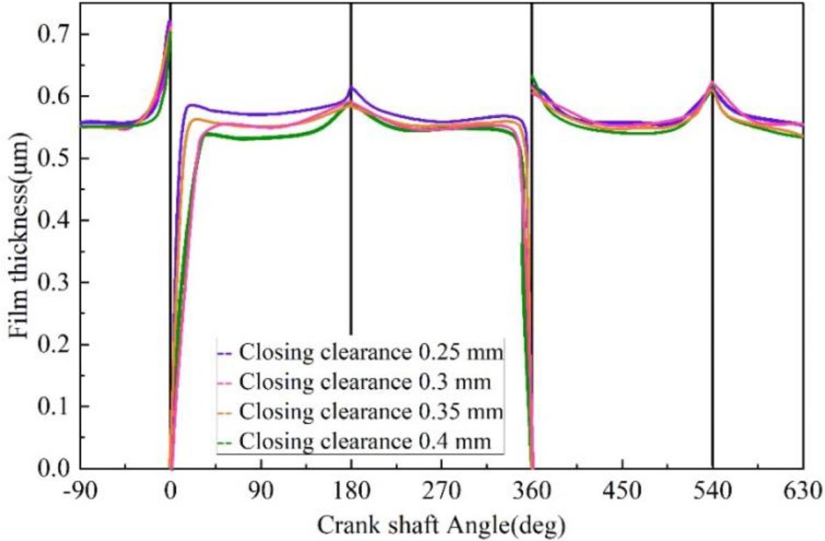
The thickness of the oil film is related to the change of the crankshaft
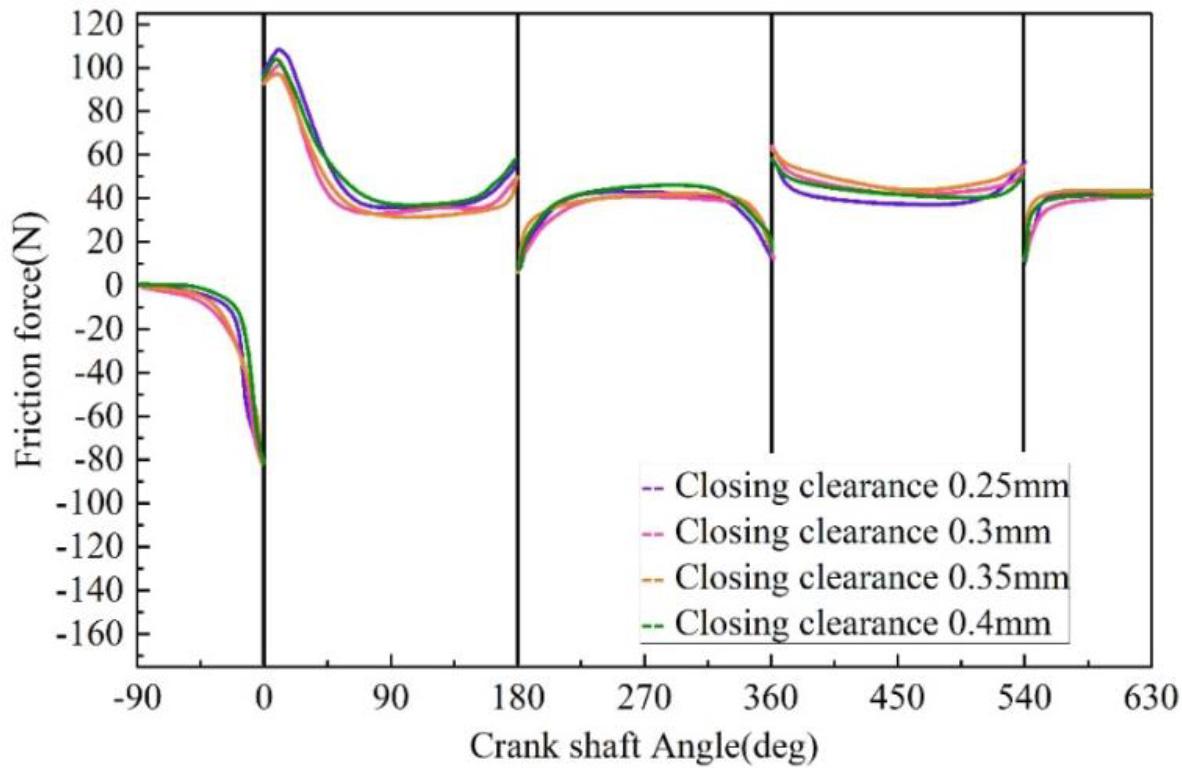
The friction of friction is related to the change of crankshaft Angle
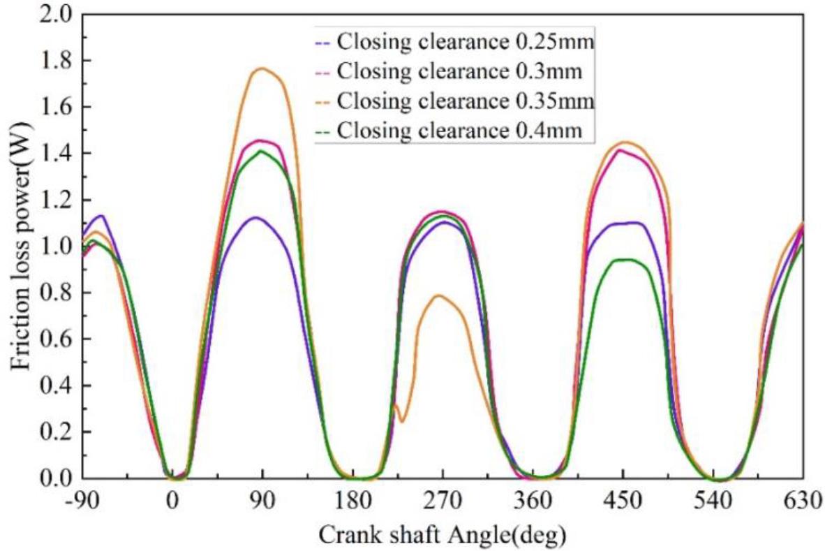
The friction loss power is related to the change of crankshaft Angle
Orthogonal testing is an efficient test design method that selects a representative part of the test program from all of them based on orthogonal design.The minimum oil film thickness and friction loss work of the piston ring are used as evaluation indexes for the orthogonal optimization test.The three structural parameters of the top ring, namely the mid-bump position, effective lubrication length, and barrel height, were used as optimization factors in the orthogonal optimization test. Table 1 displays the factor levels of the orthogonal optimization test for piston ring profile parameters for the three groups of levels designed for this orthogonal test.
| Name | Medium convex point offset | Effective lubrication length (mm) | Barrel height(μm) |
|---|---|---|---|
| Level 1 | 10% | 5 | 10 |
| Level 2 | 20% | 5.4 | 14 |
| Level 3 | 30% | 5.8 | 18 |
The optimization test of piston ring profile parameters designed in this paper has three factors and three levels, and a total of 27 groups of tests need to be done if the method of full-scale test is used, while only 9 groups of tests need to be carried out if the method of orthogonal test is used. Therefore, the orthogonal optimization test has the potential to significantly enhance the test efficiency.The greater the extreme results of the three factors of center bump position, effective lubrication length, and barrel height, the greater the influence of the factor on the evaluation index. The results of the orthogonal optimization test of piston ring profile parameters are shown in Table 2. The height of the barrel surface has the greatest influence on the minimum oil film thickness, while the effective lubrication length has the least influence. In addition, the position of the center bump has the greatest influence on the work of friction loss. The lower the combined score of each level, the better its effect on the minimum oil film thickness and friction loss work of the top ring.
| Name | Medium convex point offset | Effective lubrication length (mm) | Barrel height(μm) | Minimum oil film thickness(μm) | Friction loss work(kW) |
|---|---|---|---|---|---|
| Solution 1 | 10% | 5 | 10 | 1.912 | 0.331 |
| Solution 2 | 10% | 5.4 | 14 | 1.829 | 0.325 |
| Solution 3 | 10% | 5.8 | 18 | 1.762 | 0.332 |
| Solution 4 | 20% | 5 | 14 | 1.859 | 0.312 |
| Solution 5 | 20% | 5.4 | 18 | 1.785 | 0.309 |
| Solution 6 | 20% | 5.8 | 10 | 2.015 | 0.310 |
| Solution 7 | 30% | 5 | 18 | 1.811 | 0.280 |
| Solution 8 | 30% | 5.4 | 10 | 2.021 | 0.289 |
| Solution 9 | 30% | 5.8 | 14 | 1.965 | 0.284 |
The results of the extreme deviation of each factor and the comprehensive score of each level are shown in Table 3. From the table, it can be seen that in the analysis of the comprehensive score of each level of the top ring profile parameters, the 3rd level of the comprehensive score of the position of the center bump is the lowest, so the center bump should be designed to be shifted upward by 30%, and similarly, the optimal design of the effective lubrication length is 4.8 mm, and the optimal design of the barrel surface height is 10 μm.
| Name | Medium convex point offset | Effective lubrication length (mm) | Barrel height(μm) |
|---|---|---|---|
| Minimum oil film thickness | |||
| First level(i=1) | 1.833 | 1.849 | 1.989 |
| Second level(i=2) | 1.881 | 1.874 | 1.892 |
| Third level(i=3) | 1.934 | 1.917 | 1.78 |
| Aberration R | 0.102 | 0.064 | 0.189 |
| The friction loss of the top ring | |||
| First level(i=1) | 0.332 | 0.311 | 0.306 |
| Second level(i=2) | 0.312 | 0.324 | 0.311 |
| Third level(i=3) | 0.286 | 0.32 | 0.303 |
| Aberration R | 0.038 | 0.001 | 0.004 |
| Minimum oil film thickness | |||
| First level(i=1) | 4 | 3 | 1 |
| Second level(i=2) | 3 | 2 | 2 |
| Third level(i=3) | 2 | 1 | 3 |
| The evaluation index of the friction loss | |||
| First level(i=1) | 4 | 1 | 2 |
| Second level(i=2) | 3 | 3 | 3 |
| Third level(i=3) | 2 | 2 | 1 |
| Top ring type line parameter | |||
| First level(i=1) | 7 | 4 | 3 |
| Second level(i=2) | 5 | 5 | 5 |
| Third level(i=3) | 3 | 3 | 4 |
The best-optimized solution obtained through the orthogonal optimization test is compared with the original solution, and the results of minimum oil film thickness and friction loss work of the top ring are compared, as shown in Table 4. Compared with the original scheme, the minimum oil film thickness of the optimized scheme increases by 45.67%, and the work of friction loss decreases by 3.2%.
| Name | Medium convex point offset | Effective lubrication length (mm) | Barrel height(μm) | Minimum oil film thickness(μm) | Friction loss work(kW) |
|---|---|---|---|---|---|
| Original plan | Unbiased shift | 2.6 | 18 | 1.431 | 0.295 |
| After optimization | 35% | 4.6 | 10 | 2.051 | 0.282 |
The input variables of the prediction model were set to be the ratio of the four additives, and the output variables were the average friction coefficient and. The model prediction results were analyzed in comparison to the actual values.The prediction of the average friction coefficient is shown in Fig. 16. From the figure, the average coefficient of friction of the real value is 0.984, and the average coefficient of friction predicted by using the model of this paper is 0.994. The prediction results of the model designed in this paper are more consistent with the real value, and the deviation of predictions is smaller, which indicates that the model fitting effect is better.
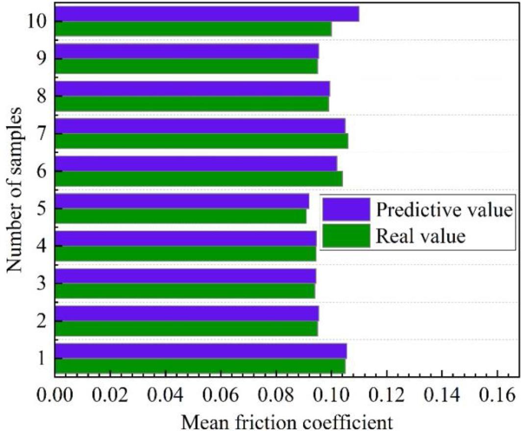
Average friction coefficient prediction
In order to further verify the reliability of the optimization scheme above, this section uses the proposed model for predicting the wear on the surface of the cylinder liner of the internal combustion engine to predict the wear on the piston rings of the cylinder liner of the internal combustion engine, which uses the optimization scheme in the previous section. The friction of the piston ring set before and after optimization is shown in Fig. 17. The friction power consumption of the piston ring set before and after optimization is shown in Fig. 18. From the figure, it can be seen that the surface wear prediction model proposed in this paper has a good prediction effect for internal combustion engine cylinder liners. The friction power of the piston ring group at the upper and lower stops is significantly improved, while the improvement of friction power at other angles of the crank angle is relatively not as obvious as that at the upper and lower stops. The friction power consumption tends to decrease throughout the cycle, especially near the upper and lower stops.
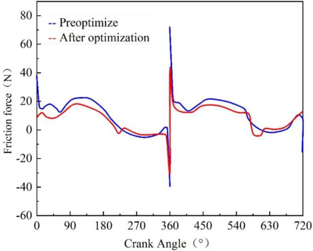
The friction of the piston ring group before and after optimization
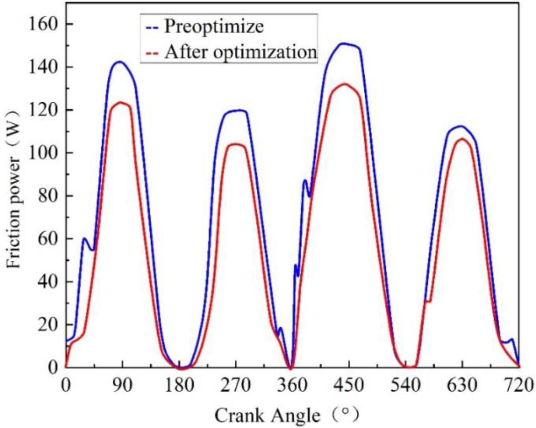
The friction power consumption of the piston ring group is optimized
The cylinder liner piston is one of the important friction factors in internal combustion engines. Its wear state directly affects the performance and life of the internal combustion engine. Therefore, this paper proposes a method for numerical simulation and performance optimization of in-cylinder friction of the cylinder liner piston ring of an internal combustion engine based on a deep neural network. Through experimental tests, this paper concludes:
In the analysis of the comprehensive score of each level of the top ring profile parameter, the 3rd level of the comprehensive score of the mid-bump position is the lowest, so the mid-bump should be shifted upward by 30%, the optimal design of the effective lubrication length is 4.8 mm, and the optimal design of the barrel surface height is 10 μm.
After analyzing the effect of the cylinder liner surface wear prediction model proposed in this paper on the internal combustion engine, it is found that the friction of the piston ring set at the upper and lower stops has a significant improvement.