Design of new energy market indicator system and dynamic risk assessment based on graph neural network: enhancing market monitoring and forecasting capability

Marketization is the best method to optimize the allocation and utilization of energy resources. With the development of the world economy, especially the acceleration of the market-oriented reform process in the world, the world’s energy use is becoming more and more market-oriented, the world’s governments intervene directly in the use of energy more and less, the energy market has become the main mechanism for the formation of energy prices.

The energy market is the carrier of the economic operation of energy commodities, is the sum of energy commodity trading relations, and is the market economic system to deal with the energy problem of institutional arrangements [18-19]. This section analyzes the world’s energy market from three levels.

Market structure refers to the basic characteristics of a market, including the number of vendors, the degree of homogeneity of the products of each vendor, and the ease of entry and exit from the market. In economics, there are typically four market structures. Monopolistically Competitive Markets, Oligopolistic Markets, Perfectly Competitive Markets, and Perfectly Monopolistic Markets. However, the international energy market has a complex market structure.

With the increase in membership, OPEC has developed into an international oil organization for some of the major oil-producing countries in Asia, Africa, and Latin America. With annual OPEC crude oil production accounting for 40 per cent of total global production and exports accounting for 55 per cent of the world’s total trading volume, it is clear that this is an oligopolistic market structure with a high rate of concentration. After nearly 40 years of development, OPEC has become an important force to be reckoned with in the international energy market. The complexity of the energy market structure is also reflected in the struggle between monopolies and non-monopolies.

Since the equilibrium price in the energy market has a continuous upward trend in the long run, it is determined that the real energy price must also have a long-term upward trend. In the short term, there are a variety of factors that affect the short-term trend of energy market prices.

The risk of price volatility in the energy market refers to the possibility of drastic, substantial, and unpredictable changes in prices. Energy market risk management research is usually directly applied to the methods and models based on financial markets, but in fact, the energy market risk has its special characteristics, and the traditional methods cannot fully meet the needs of energy market risk management.

The volatility of the market price represents the risk of the oil market, and the transaction represents the realization of the risk. In this link, the traders are essentially exchanging the use value of oil, along with the transfer of ownership of the physical commodity. In some cases, the transfer of ownership of energy assets does not occur, such as the storage and transportation process of oil also takes a long time, but the corresponding types of cost constraints of energy assets are always in a reasonable commercial process.

In view of this, this paper proposes a holistic definition of risk. By risk, we mean exposure to various risk elements, such as objective probability and time. “Objective probability” is the statistical significance of the likelihood of the outcome of the event, and “time” is the statistical significance of the evolution of things brought into the possibility of change. These two elements have universal, objective, and common characteristics. “Exposure” is the state of the subject of risk, which is localized, subjective and individual, depending on the subject of risk-taking. Objective probability and time constitute a kind of subjective probability space.

The transfer of information between financial markets can be seen as the impact of changes in one economy on other economies. With the deepening of the degree of information technology between markets, the speed of information transfer between the economies of the markets is also increasingly accelerated. In order to explore the correlation between the transfer of information between markets, many scholars have begun to use the term “spillover effect” to express the relationship between the transfer of information between markets. Therefore, the risk spillover effect can be expressed as follows: in the process of information transfer between different markets, when the asset price of a market is affected by the information changes, it further leads to other market asset prices also affected by the impact of the information and change. This cross-transmission of information between different markets is the risk spillover effect between markets.

Risk spillovers have four basic characteristics: negative contagion, negative externality, accumulation, and risk-return asymmetry.Contagion refers to the fact that when a risk arises in one market, it is transmitted from that market to other markets. Negative externalities refer to the corresponding spillover of risk through inter-market correlations when risk arises in one market and leads to the accumulation of market externalities. Accumulation refers to the further accumulation of risk, e.g., when the risk occurs in market X, causing sharp price fluctuations, it also causes price fluctuations in market Y, and price fluctuations in market Y, in turn, further affect market X, and so on, further accumulating inter-market risk. Markets generate different risk premiums in response to risk, creating operational risks and economic losses between them, which is known as risk-return asymmetry.

In the study of risk transmission in energy financial markets, risk transmission between the oil market and the stock market and exchange rate market is a complex process, which not only needs to take into account the characteristics of non-linearity, multi-timescale, and asymmetry of cross-market inter-risk transmission, but also it is crucial to choose the appropriate samples and methods to conduct the related research.

The research related to risk transmission in energy financial markets conducted in this paper mainly refers to the mutual transmission of risk between energy financial markets and major financial markets. It is worth noting that risk transmission in the context of the financial crisis is an integral part of risk transmission in energy financial markets, which means that risk transmission in energy financial markets includes risk transmission in the context of the financial crisis. The financial crisis is, to some extent, a product of the continuous accumulation of financial risks. The financial crisis stage is considered to be the outbreak stage of financial risks, and the risks after the outbreak continue to spread and spread to various markets, that is, the risk transmission stage of the financial crisis.

The energy financial market is a new type of trading market that is based on the integration of the energy and financial markets.The close connection between energy financial markets and traditional financial markets will only strengthen, not weaken.Energy financial markets are not only affected by risk spillovers from related markets, but they cannot avoid transmitting risks to other markets related to them.

Value at Risk (VaR), VaR is a means of quantitatively assessing risk. Its formula is expressed as follows: (1) VaR(X)α=inf{(x|f(X<x))≤1−α} \[VaR{{(X)}_{\alpha }}=inf\{(x|f(X<x))\le 1-\alpha \}\] Where α is generally taken as 0.05 or 0.01, 1–α is the confidence level, x is the sequence of returns on the asset or portfolio, and f(x) is the probability distribution function of the returns. The essence of VaR is to calculate the number of the tails of the random distribution of returns.

Expectation Shortfall (ES): ES indicates the average degree of loss suffered when the portfolio loss exceeds the VaR threshold. Its formula is expressed as in equation (2): (2) ES(X)α=E[X|X≥VaR(X)α] \[ES{{(X)}_{\alpha }}=E[X|X\ge VaR{{(X)}_{\alpha }}]\]

ES essentially calculates its conditional expectation for extreme values greater than VaR. By taking into account the mean level of the extremes on top of the VaR, it is more reflective of the risk characteristics of the portfolio or asset and is better suited to expressing tail risk.

Generalised Autoregressive Score (GAS) models are also known as dynamic conditional score models. This is because GAS models are able to capture the complexity and non-linear relationships in the time series, thus more accurately describing future trends. It provides a new option for modelling the volatility of financial asset returns.

Assuming y_i is a financial time series observation, f_t−1 is the information set at moment t–1, the set of instantaneous parameters, Xⁿ is a vector of exogenous variables, and ϕ is a static parameter variable, the probability density function of observation y_i is as follows: (3) p(yt|ft−1,Xt,ϕ) \[p({{y}_{t}}|{{f}_{t-1}},{{X}^{t}},\phi )\]

The probability density function can account for the fact that the observed information at moment t–1 becomes the observation-driven probability density function at moment t , and thus the parameter changes in the GAS model are data-driven dynamic processes. It can be expressed as: (4) ft=w+∑i=0pAist−i+∑j=1qBjft−j \[{{f}_{t}}=w+\sum\limits_{i=0}^{p}{{{A}_{i}}}{{s}_{t-i}}+\sum\limits_{j=1}^{q}{{{B}_{j}}}{{f}_{t-j}}\]

Among them: (5) { st=St∇t∇t=∂lnp(yt|ft−1,Xt,ϕ)∂ft−1St=It−γ=Et−1[∇t∇t′] \[\left\{ \begin{matrix} {{s}_{t}}={{S}_{t}}{{\nabla }_{t}} \\ {{\nabla }_{t}}=\frac{\partial \ln p({{y}_{t}}|{{f}_{t-1}},{{X}^{t}},\phi )}{\partial {{f}_{t-1}}} \\ {{S}_{t}}=I_{t}^{-\gamma }={{E}_{t-1}}[{{\nabla }_{t}}\nabla _{t}^{\prime }] \\ \end{matrix} \right.\] Where A_i and are B_j time-varying coefficient matrices, where i = 1,2,…,p, j = 1,2,…,q , reflect the time-varying nature of the fluctuations and the aggregation of the fluctuations, respectively, and usually it is sufficient to take 1 for p and q . w is a constant vector, reflecting the mean reversibility.

The multivariate Student’s t-distribution, based on a mixture of multivariate normal and cardinal distributions, has a wider range of applications and greater flexibility, and compared with the multivariate normal distribution, it can better capture outliers, sharp peaks, thick tails and other features in the financial time series, which demonstrates its superiority. Let y be an k-dimensional random variable and the probability density function of the multivariate student t distribution is equation (6): (6) F(y|μ,Σ,ν)=Γ((ν+k)/2))|Σ|−1/2Γ(ν/2)[1+(y−μ)TΣ−1(y−μ)](ν+k)/2(πν)k/2 \[F(y|\mu ,\Sigma ,\nu )=\frac{\Gamma ((\nu +k)/2))|\Sigma {{|}^{-1/2}}}{\Gamma (\nu /2){{[1+{{(y-\mu )}^{T}}{{\Sigma }^{-1}}(y-\mu )]}^{(\nu +k)/2}}{{(\pi \nu )}^{k/2}}}\] Where μ is the location parameter, Γ(·) is the gamma function, Σ is the k -dimensional covariance matrix, and ν is the degrees of freedom of the multivariate Student t distribution.

In rolling estimation, using matrix H_t to represent the eigenvalues of the covariance matrix Σ , and the eigenvectors of the covariance matrix Σ_i, the covariance matrix Σ_i can be expressed in the following form: (7) Σt=DtHtDt′ \[{{\Sigma }_{t}}={{D}_{t}}{{H}_{t}}D_{t}^{\prime }\] Where D is an orthogonal matrix, i.e. Di*Di′=I$D_{i}^{*}D_{i}^{\prime }=I$ , I are unit matrices. D_t is a diagonal matrix whose elements on the diagonal are the eigenvalues of the covariance matrix H_t indicating the magnitude of volatility of different random variables. The volatility σ_i can be expressed as: (8) σt=νν−2tr(Σt)k \[{{\sigma }_{t}}=\sqrt{\frac{\nu }{\nu -2}}\sqrt{\frac{tr({{\Sigma }_{t}})}{k}}\] Where tr(Σ_i) denotes the trace of the covariance matrix.

The estimation of dynamic correlation coefficients using the multivariate GAS model is similar to the generalised dynamic conditional correlation coefficient (DCC-GARCH) model. Assuming that the distribution is a multivariate student t-distribution for multidimensional when taking two random variables y_i and y_j as an example. The covariance matrix Σ_t is estimated based on the GAS model to expand the multivariate student t distribution (yi,t−μi,t)TΣi,t−1(yj,t−μj,t)${{({{y}_{i}},t-{{\mu }_{i,t}})}^{T}}\Sigma _{i,t}^{-1}({{y}_{j,t}}-{{\mu }_{j,t}})$ is obtained: (9) (yi,t−μi,t)TΣij,t−1(yj,t−μj,t)=∑i=1k∑i=1k(yi,t−μi,t)Σij,t−1(yj,t−μj,t) \[{{({{y}_{i,t}}-{{\mu }_{i,t}})}^{T}}\Sigma _{ij,t}^{-1}({{y}_{j,t}}-{{\mu }_{j,t}})=\sum\limits_{i=1}^{k}{\sum\limits_{i=1}^{k}{({{y}_{i,t}}-{{\mu }_{i,t}})}}\Sigma _{ij,t}^{-1}({{y}_{j,t}}-{{\mu }_{j,t}})\]

Their correlation coefficients are calculated as follows: (10) ρij,t=Σij,t/Σii,tΣjj,t \[{{\rho }_{ij,t}}={{\Sigma }_{ij,t}}/\sqrt{{{\Sigma }_{ii,t}}{{\Sigma }_{jj,t}}}\] Where Σ_ij,t denotes the i th row and j th column elements of the t-moment covariance matrix Σ_i.

The correlation coefficient ρ_ij,t is brought into the expanded equation (11) to obtain: (11) (yi,t−μi,t)TΣij,t−1(yj,t−μj,t)=∑i=1k(yi,t−μi,t)2+∑i≠jΣi,tΣi,tΣj,t(yi,t−μi,t)(yj,t−μj,t) \[\begin{align} & {{({{y}_{i,t}}-{{\mu }_{i,t}})}^{T}}\Sigma _{ij,t}^{-1}({{y}_{j,t}}-{{\mu }_{j,t}})=\sum\limits_{i=1}^{k}{{{({{y}_{i,t}}-{{\mu }_{i,t}})}^{2}}} \\ & +\sum\limits_{i\ne j}{\frac{{{\Sigma }_{i,t}}}{\sqrt{{{\Sigma }_{i,t}}{{\Sigma }_{j,t}}}}}({{y}_{i,t}}-{{\mu }_{i,t}})({{y}_{j,t}}-{{\mu }_{j,t}}) \\ \end{align}\]

The final dynamic correlation coefficient based on the GAS model can be expressed as: (12) pij,t=∑i≠jΣij,tΣii,tΣij,t(yi,t−μi,t)(yj,t−μj,t)∑i=1k(yi,t−μi,t)2∑j=1k(yj,t−μj,t)2 \[{{p}_{ij,t}}=\frac{\sum\limits_{i\ne j}{\frac{{{\Sigma }_{ij,t}}}{\sqrt{{{\Sigma }_{ii,t}}{{\Sigma }_{ij,t}}}}}({{y}_{i,t}}-{{\mu }_{i,t}})({{y}_{j,t}}-{{\mu }_{j,t}})}{\sqrt{\sum\limits_{i=1}^{k}{{{({{y}_{i,t}}-{{\mu }_{i,t}})}^{2}}}\sum\limits_{j=1}^{k}{{{({{y}_{j,t}}-{{\mu }_{j,t}})}^{2}}}}}\] Where the numerator is the sum of the products of the off-diagonal elements of the covariance matrix and the sample points away from the mean, and the denominator is the square root of the product of the sum of the squares of the sample points away from the mean.

Conditional at-risk value (CoVaR), which measures the impact of subsystems on total system risk when they are in crisis. The CoVaRa[ψ]$CoVaR_{a}^{[\psi ]}$ essence represents the maximum possible loss to system i when system j is at the extreme, i.e., when system j has a return of VaRaj$VaR_{a}^{j}$ the level of risk that is i at j risk under insured conditions. The expression is given below: (13) prob(y≤CoVaRα4j|y≤VaRαj) \[prob(y\le CoVaR_{\alpha }^{4j}|y\le VaR_{\alpha }^{j})\]

In the framework of the GAS model, the dynamic correlation coefficients have been calculated and, according to equation (13), the expressions for VaR and CoVaR can be written as equations (14) and (15), respectively: (14) VaRα,ji=uii−qα,jhii \[VaR_{\alpha ,j}^{i}=u_{i}^{i}-{{q}_{\alpha ,j}}h_{i}^{i}\] (15) CoVaRα,tij=VaRα,ti(σti1−(ρtij)2+ρtijσtj) \[CoVaR_{\alpha ,t}^{ij}=VaR_{\alpha ,t}^{i}(\sigma _{t}^{i}\sqrt{1-{{(\rho _{t}^{ij})}^{2}}}+\rho _{t}^{ij}\sigma _{t}^{j})\] Where uii$u_{i}^{i}$ is the conditional mean, q_a,j is the value of the quantile of the probability distribution that system i returns obey, and hii$h_{i}^{i}$ is the conditional standard deviation of the returns in the GAS model. σti\[\sigma _{t}^{i}\] and σtj\[\sigma _{t}^{j}\] are the volatilities of system i and system j at moment t, respectively.

The risk premium of system j over system i is specified as the formula: (16) ΔCoVaRα,ti|j=CoVaRα,ti|j=VaRαγ−VaRα,ti \[\Delta CoVaR_{\alpha ,t}^{i|j}=CoVaR_{\alpha ,t}^{i|j=VaR_{\alpha }^{\gamma }}-VaR_{\alpha ,t}^{i}\]

Financial institutions can use ΔCoVaR to assess the effectiveness of their hedging strategies, for example, when using options or other derivatives to hedge risk, and can use ΔCoVaR to measure possible risk exposures and the effectiveness of hedging. And they can use ΔCoVaR to conduct risk stress tests to test the exposure of their portfolios under different market conditions.

In order to compare the risk spillover contribution of different systems to system i , the risk spillover values are de-measured in the empirical evidence and the risk spillover contribution is defined as % ΔCoVaRai|j$\Delta CoVaR_{a}^{i|j}$ as follows: (17) %ΔCoVaRαi|j=ΔCoVaRαi|j=VaRανVaRαi*100 \[\% \Delta CoVaR_\alpha ^{i|j} = {{\Delta CoVaR_\alpha ^{i|j = VaR_\alpha ^\nu }} \over {VaR_\alpha ^i}}*100\]

In this paper, the daily closing prices of carbon emissions trading in Shenzhen and Hubei are selected as representative products of China’s carbon market. The power coal industry index compiled by CITIC Securities Company is selected as a representative product of the coal market, and the daily closing price of the crude oil spot in Daqing is selected as a representative product of the crude oil market, and the coal market and the crude oil market are selected as representative products of the traditional energy market. The daily closing price of the CSI New Energy Index (399808) is selected as the representative product of the new energy market.Carbon market data and new energy market data are available from the Wind database, while traditional energy market data is available from the Choice database.The selected data sample interval is from January 8, 2015 to October 20, 2023.

The GARCH model can comprehensively portray the volatility of the yield series, thereby analysing the problems. The data has been tested to determine the existence of the ARCH effect in the yield series, so this paper uses the GARCH (1,1) model to test and analyse, effectively eliminating the conditional heteroskedasticity. The results of parameter estimation of the GARCH model are shown in Table 1, which shows the Akaike Information Criterion (AIC) and Bayesian Information Criterion (BIC). The AIC and BIC values of the new energy market are 3.9865 and 3.8714, respectively. And α + β < 1 holds for all five series, which can be used as an important indicator of the goodness of fit of the GARCH model.

The Ljung-Box Q test for the GARCH(1,1) model is shown in Table 2. The Ljung-Box Q test on the residual series of the GARCH(1,1) model aims to assess the presence of autocorrelation in the residuals of the model and thus, indirectly detect the presence of heteroskedasticity. The original hypothesis (H0) was the absence of autocorrelation in the residual series. The test results show that for all five return series, the statistics of the Ljung-Box Q test are greater than the critical value corresponding to the 1% significance level. The Ljung-Box Q-test p-value for the new energy market is 0.3641, and the p-values are all well above the 0.05 level of significance. This means that there is not enough evidence to reject the original hypothesis, leading to the conclusion that there is no significant autocorrelation in the residual series of the GARCH(1,1) model, suggesting that the model effectively eliminates heteroskedasticity.

Combining the results of the Ljung-Box Q-test and other statistics (AIC, BIC, etc.), it can be concluded that the GARCH(1,1) model has good robustness. Therefore, the model is suitable for use in the calculation of Value at Risk (Va R) at a later stage and provides a reliable tool for financial risk management.

In order to simplify the risk spillover effect between the Chinese carbon market and the new energy market, a similar weighting calculation method between the Chinese carbon market and the traditional energy market is adopted to derive the risk spillover value between the Chinese carbon market and the new energy market, which can more accurately determine the risk level between the Chinese carbon market and the new energy market.

The risk spillover values (q=0.05) of the carbon market and energy market are shown in Table 5. According to the direction of the spillover, the spillover effect between the carbon market and the new energy market is a bidirectional spillover that also shows bidirectional characteristics, but the dynamics are different compared with the traditional energy market. The risk spillover from the new energy market to the carbon market (16.35 per cent) is significantly higher than the spillover from the carbon market to the new energy market (7.86 per cent). This phenomenon reflects the fact that, given the accelerated global transition to sustainable energy, turbulence in the new energy market is likely to have a more significant impact on the carbon market.

In summary, it can be seen that, regardless of the direction of risk transmission, the risk spillover effect between the new energy market and the carbon market is smaller than that between the traditional energy market (e.g., coal and crude oil markets) and the carbon market. This phenomenon reveals an important substitution effect, i.e., with the development and application of new energy technologies, the new energy market is gradually replacing the traditional energy market, thus reducing the carbon market’s dependence on the traditional energy market. The existence of this substitution effect is reflected not only in quantitative indicators of risk spillover but also in changes in global energy consumption and investment trends.

Factors affecting the volatility of new energy prices are numerous and complex, and the study and analysis of factors affecting the volatility of new energy prices can effectively control the sources of risk in the new energy price market. Influencing factors can be divided into deterministic risk factors and uncertainty risk factors according to their frequency and whether they lead to the inevitable occurrence of risk.

In this paper, the study of new energy price volatility risk factors will also include deterministic and uncertainty factors. Deterministic risk factors are mainly divided into supply and demand factors, cost factors, and economic factors.

The appropriateness of the selection of evaluation indicators will affect the evaluation results to a greater or lesser extent. If there are more evaluation indicators, there will be duplications between indicators and cross-inclusive relationships between certain indicators, and if there are fewer evaluation indicators, they will not be representative, affecting the comprehensiveness of the results. There are many factors to be considered in evaluating the risk of volatility of China’s major energy prices, and these risk factors affect and constrain each other, so whether or not a scientific and reasonable evaluation indicator system can be established relates to whether or not it can play a role in the evaluation. In order to ensure that the evaluation index system has the expected effect, it is important to follow the following four basic principles when establishing it.

Following the above 4 principles, this paper adopts a comprehensive evaluation method for the risk of new energy price fluctuations, taking supply and demand factors, economic factors, cost factors, and uncertainty factors as a total of 4 risk factors as primary indicators. The corresponding 12 secondary indicators are selected as measurement variables to establish the new energy price volatility risk evaluation index system.

The new energy price fluctuation risk evaluation index system is shown in Figure 1. The supply and demand factors include energy storage and extraction ratio, energy supply and demand ratio, and external dependence on energy. Economic factors include industrial value added, GDP growth rate, and US dollar exchange rate. Cost factors include production costs, transportation costs, and safety costs.Uncertainty can be caused by emergencies, national policies, and natural disasters.

Figure 1.

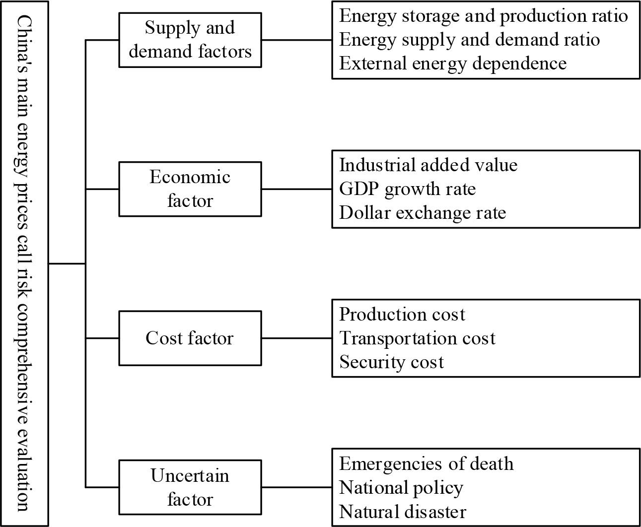
New energy price fluctuation risk evaluation index system

In this paper, nine indicators, namely COMEX gold, Euro RMB exchange rate, Yen RMB exchange rate, USDX US Dollar Index, WTI crude oil, Hong Kong Dollar to RMB exchange rate, US Dollar to Hong Kong Dollar, Pound Sterling to RMB exchange rate, and Shanghai Stock Exchange 50 Index, are finally selected as research objects. Since more data is needed for forecasting, this paper selects the daily closing prices of these nine indicators from 2015 to 2023 as the self-knowledge data for forecasting.These nine indicators are processed using upper and lower mean padding methods and descriptive statistics on risk.

In this paper, GRU units in graph convolutional neural networks and recurrent neural networks are used to forecast the nine financial indicators. The Pearson correlation coefficient between indicators is used to construct the graph structure in graph convolutional neural networks. For the Pearson correlation coefficient greater than 0.8, this paper considers that there is a correlation between the two variables, and the value of the element in the corresponding position of the neighbour matrix is 1. For the value of the Pearson coefficient less than 0.8, the value of the corresponding element of the neighbour matrix is 0. The calculation method of the elements of the neighbour matrix is shown below: (33) Ai,j={ 1, if ρ >0.80, if ρ≤0.8 \[{{A}_{i,j}}=\left\{ \begin{align} & 1,\text{ if }\rho \text{ 0}\text{.8} \\ & 0,\text{ if }\rho \le \text{0}\text{.8} \\ \end{align} \right.\]

In order to better compare the prediction performance of this paper’s method on a variety of amount indicators, this paper chooses Long Short-Term Memory Neural Network (LSTM), Random Forest, and XGBoost to compare with this paper’s method. In this paper, the mean absolute error, mean absolute percentage error, and root mean square error are chosen as statistical indicators.

In this section, the energy stock price of GNN SSE 50 calculated by the GRU unit is used to predict the value of the next day by analyzing historical data from the previous 12 days.X is the input data, the number of rows is the number of financial indicators, and the number of columns is the number of input times.In this paper, 9 financial indicators are used to predict the value of the next point in time using the values of the previous 12 inches. Therefore, X is a matrix with 9 rows and 12 columns.

To better illustrate the excellent performance of the methods used in this paper, LSTM, Random forest, and XGBoost are used to compare with the methods in this paper. The GNN constructed in this paper uses 300 hidden units with a batch size of 64. The learning rate is 0.002 and the number of training times is 500. The LSTM used is a two-layer LSTM with a Dropout before the output layer to prevent overfitting. The Dropout Rate set is 0.5.

Random forest is an integrated algorithm that consists of multiple decision trees and no association between the decision trees that do not pass.Random forest is a commonly used machine learning model for both classification and regression problems. The number of Random Forest trees used in this paper is 30. XGBoost is also known as an extreme gradient boosting tree. It is an implementation of a boosting algorithm. The number of trees is 300, and the maximum depth is 6. In this paper, 95% of the data is used for training, and the remaining 85 samples are used as the test set.Table 6 displays the prediction errors of various methods for the SSE 50 index.

It can be seen that among several machine learning models, GNN achieves the highest prediction accuracy for stock prices, and its performance outperforms other models by at least 20%. Meanwhile, this paper also selects and replaces the parameters of various estimation methods and finds that none of them exceeds the accuracy of GNN. Therefore, GNN has the highest prediction accuracy among all the models.

After constructing the new energy financial market risk early warning model, the sample data interval selected in this paper is the daily data of WTI crude oil futures yield from 2015 to 2023 to verify the validity of the model. Among them, the data from the first 50 months is the training set, and the data from the latter month is the test set.

The new energy financial risk early warning model constructed in this paper is compared and analysed with other prediction models in order to prove that the prediction performance of the graph neural network-based prediction model in this paper is better than that of other prediction models.

The results of the comparative analysis between the new energy financial risk early warning model proposed in this paper and other prediction models are shown in Table 7. Among them, the comparative models include single support vector machine model (SVM), multivariate grey prediction model (GM(1, N)), multivariate autoregressive sliding average model (ARMAX), BP neural network prediction model (BP), and multivariate regression model (RM) Specific analyses of the results are as follows.

The prediction based on the graph neural network is significantly better than the other comparative prediction models, with the values of MAPE, MAE, and RMSE of 3.52%, 0.756, 0.598, and the prediction validity of 0.891, respectively. In terms of the different orders, the first order denotes the prediction by using one period of lagging of the influencing factors. Similarly, the fourth order indicates a prediction using a lag of four periods for the influencing factors.Obviously, all the indicators show that the prediction effect of energy financial risk warning using lag one of the influencing factors is better than the prediction effect of lag two, lag three, and lag four. The difference between MAPE, MAE and RMSE in lag one and lag four is 2.02, 0.598 and 0.299, respectively, and the difference in predictive validity is 0.177, which is a big difference in all four indicators. Because the new energy financial market risk and impact have a close linkage, that is, when the macro economy or new energy market and other risks occur, it will soon be able to be transmitted to the new energy financial market, triggering the price fluctuations of the new energy financial market, which in turn generates risk. Therefore, when any influencing factors related to the new energy financial market change, the new energy financial market is likely to be at risk and needs to be warned early.

For different types of multifactor prediction models, SVM has the highest prediction accuracy, GM(1, N) has the second highest prediction accuracy, followed by ARMAX, then the multiple regression model and the worst prediction accuracy is the BP neural network model.

In summary, based on the results in the table, the following conclusions can be drawn.

One, the new energy financial risk early warning model based on the graph neural network used in this paper has the highest prediction accuracy as well as prediction validity, and the model is able to effectively capture the linear and nonlinear characteristics of energy financial market prices.

Second, the prediction performance of the combined prediction model is better than that of individual prediction models.

Third, for the new energy financial risk market, the prediction method based on machine learning and statistical theory is better than a single prediction model based on artificial intelligence or a single prediction model based on statistical measurement theory.