Research on deep learning image segmentation method based on attention mechanism

Online veröffentlicht: 17. März 2025
Eingereicht: 24. Okt. 2024
Akzeptiert: 12. Feb. 2025
DOI: https://doi.org/10.2478/amns-2025-0210
Schlüsselwörter
© 2025 Haibo Li, published by Sciendo
This work is licensed under the Creative Commons Attribution 4.0 International License.
Attention mechanism refers to the fact that when human beings receive external information, after certain filtering, processing and selection, they focus their attention on the important information, process and memorize it, while ignoring the irrelevant information. It is one of the bases for human beings to acquire knowledge and perceive the world, and it is also one of the important research directions in the field of artificial intelligence [1-4]. Image segmentation refers to dividing the pixels in a digitized image into different regions and assigning a label to each region, such as foreground, background, object, and so on. Currently, image segmentation techniques have been widely used in various fields, such as medical imaging, natural image processing, face recognition, intelligent transportation systems and robotics [5-8]. Traditional image segmentation methods are mainly based on features such as pixel color information, texture information and edge information, and these methods will fail in complex situations. And deep learning based image segmentation algorithms are increasingly used for their excellent performance and high accuracy [9-12].
In recent years, the application of deep learning techniques in the field of image processing has made great progress, especially in image segmentation and analysis. Deep learning-based image segmentation techniques can automatically divide a digitized image into several non-overlapping regions and assign each region with a corresponding semantic label [13-16]. It is robust and adaptable and can be used for a variety of different types of images, such as medical images and nature images. Currently, there are three main approaches for deep learning based image segmentation techniques, namely FCN, U-Net and MaskR-CNN [17-20].
This paper provides a brief overview of deep learning techniques and attention mechanism based on the image segmentation technology framework of deep learning. In order to further improve the quality and efficiency of image segmentation, the encoder-decoder idea is utilized to construct the feature fusion network (TCNet) with large convolutional kernel and attention mechanism. An image segmentation network incorporating four parts: large convolutional kernel module (LKM), enhanced transformer module (ETM), multi-scale feature fusion module (MFM) and decoder is designed. Set up the experimental environment as well as the loss function, and analyze the values of the loss function parameters. Select several datasets to compare the performance indexes of classical image segmentation algorithms and obtain the image segmentation performance of the TCNet method designed in this paper.
Image segmentation can be divided into three main categories, semantic segmentation, instance segmentation and panoramic segmentation. As a common sense image segmentation generally means semantic segmentation, which provides not only category prediction but also spatial location information of these categories by categorizing all pixel points on a picture. Image semantic segmentation can be viewed as a pixel-level classification task where each pixel is labeled and classified into a specific category by densely predicting and inferring labels for each pixel. Instance segmentation is a combination of target detection and semantic segmentation to achieve edge segmentation of an object, resulting in a single segmentation instance. As opposed to semantic segmentation, instance segmentation is segmenting a single object and labeling it. Panoramic segmentation is a recently developed segmentation task that can be represented as a combination of semantic and instance segmentation.
In recent years, deep learning technology has been rapidly developed and has been widely used in computer vision, image processing, natural language processing and other fields. Different from traditional machine learning algorithms in large-scale data and complex scenes, deep learning algorithms are able to directly use the raw data as input to the model, and utilize the multi-layer network structure in the network model to transform the input data into high-level abstract feature expressions. This enables the extraction of data features. The advantage of this algorithm is that it can realize the extraction of data features and there is no human intervention in the learning process of the model in order to improve the fitting ability of the model and improve the processing effect of the algorithm.
The nature of the attention mechanism is a weighted summation operation that aims to make the model more focused on the more important parts of it [21-22]. In general, the attention mechanism consists of three main steps. The first is the calculation of attention weights, by which the attention weights of different positions are calculated in some way to express the degree of importance between them. The second is weighted summation, which weights and sums the information according to the attentional weights. The third is updating the model, where the weighted summation results are federated with the output of the original model in order to update the model. Common attention mechanisms include global attention, local attention, self-attention, etc. Different attention mechanisms are applicable to different scenarios and tasks.
The attentional mechanism works to amplify the weights of useful information and minimize the weights of useless information. The elements in the data are constructed into a series of 〈
where
Self-attentive mechanisms are a recent scientific advance in obtaining long-range interactivity, but are still mainly used only for sequence modeling and generative modeling tasks. The key idea behind the self-attention mechanism is to obtain a weighted average of the values computed by the hidden units. Unlike pooling or convolution operators, the weights used in the weighted average operation are obtained dynamically through a similarity function between the hidden units. As a result, the interaction between the input signals depends on the signals themselves, rather than being predetermined by their relative positions. It is worth mentioning that this allows the self-attentive mechanism to obtain long-term interactivity without increasing the parameters.
The self-attention mechanism is based on an improvement of the attention mechanism, which is better at capturing the internal relevance of the data or features. A larger sense field and more contextual information is obtained by capturing the global information. The self-attention mechanism provides a modeling way to efficiently capture global contextual information through the triad of (
where
In this study, we construct a large convolutional kernel and attention mechanism feature fusion network (TCNet) based on the idea of encoder-decoder, which consists of four parts: a large convolutional kernel module (LKM), an augmented Transformer module (ETM), a multiscale feature fusion module (MFM), and a decoder.
The receptive field is a key factor that affects the network to extract the complete shape information of the image or region of interest, in order to expand the effective receptive field (ERF) of the network more effectively, this study has done an in-depth exploration on the extra-large convolutional kernel. Equation
The large convolutional kernel module, i.e., LKM, contains two BN-Conv sequences, two 1×1 dense convolutional layers and one 31×31
In Eq. (3),
After that, the feature map
In Eq. (5), Conv denotes the 1×1 dense convolution operation, DW is the very large convolutional layer, and the symbol ⊕ denotes the channel splicing operation.
Subsequently feature map
where
The activation function processed feature maps are fed into the last 1×1 dense convolutional layer to produce the feature map
Inspired by the outstanding performance of the visual Transformer in modeling distant pixel relationships, the Enhanced Transformer Module (ETM) is designed in this paper. It uses a DW mega-convolution kernel as the core component to perform convolution operations, which, combined with a multi-head self-attention mechanism, can further address the problem of incomplete labeling in images due to sensory field constraints.
The ETM contains a similar structure for the upper and lower parts, each of which consists of three layer normalization (LN) layers, one multinomial self-attention layer, one 31×31
In order to effectively fuse the multi-scale feature maps produced by the large convolutional kernel CNN branch and the augmented Transformer branch, the multi-scale fusion module (MFM) is designed in this study. The feature maps generated by the large convolutional kernel CNN branch contain complete shape information, while the feature maps output from the augmented Transformer branch are rich in remote pixel dependencies. Therefore, the MFM, which combines the multi-scale fusion mechanism and the multi-head self-attention mechanism, can be used as a bridge to effectively fuse the two feature maps.
The MFM processes the feature maps to be fused in the upper, middle and lower branches. For the middle branch, the output feature maps
The two methods, average pooling and maximum pooling, generate two different spatial context descriptors,
where
For the downward branching, the maximum pooling and convolution operations are first performed on the feature map L to increase the feature channels. Then the feature map is fed into the spatial attention block to generate a spatial attention map using the spatial relationships of the features. Finally, the feature map
Eventually, the three types of feature maps
In this paper, the proposed deep learning image segmentation technique with the addition of an attention mechanism is applied to the field of medical images to test the feasibility and applicability of the technique.
The hardware and software environments used in the experiments are shown in Table 1.
The hardware and software environment of the experiment
| Central processor | Intel(R)Core i7-8600K CPU@3.60 GHz |
|---|---|
| Graphics card | Nvidia TITAN Xp 24GB |
| Memory | 64GB |
| Operating system | Windows 10 |
| Python | 3.9.15 |
| CUDA | 11.6 |
| torch | 1.13.0+cu116 |
| torchvision | 0.14.0+cu116 |
| Simulation platform | PyCharm |
In order to improve the computational efficiency, all the images are resized to 448×448, in addition to vertical flip, horizontal flip, diagonal flip, random shift and random scale change data enhancement operations are done.
In this paper, the optimal training parameters are obtained based on multiple training. This includes epoch set to 120, training batch set to 15, and model training optimized using Adam optimizer. Since too large a learning rate in the late stage of training will lead to instability of the model, while too small a learning rate will lead to a decrease in learning efficiency. Therefore, in this paper, a cosine annealing strategy is used to adjust the learning rate of the network. It essentially adjusts the learning rate curve to a cosine function model that decreases with the number of training sessions.
where
In order to fully evaluate the effectiveness of the model, five parameters, accuracy (AC), sensitivity (SE), specificity (SP), Jaccard’s coefficient (JA), and Dice’s coefficient (DI), are used in this paper for comparison. Of these, accuracy is the most intuitive metric, indicating the percentage of correctly classified pixels over all pixels. Sensitivity (also known as recall) indicates the percentage of recognized correct samples to the actual correct samples, through which you can view the segmentation results of positive samples. Specificity, on the other hand, indicates the percentage of negative samples identified versus the overall negative samples. Jaccard’s coefficient and Dice’s coefficient are used to compare the difference between the model segmented samples and the actual labeled samples, with higher scores indicating that the results of the two are more similar.
It is worth noting that in the ablation experiments, all five metrics are used in this paper. However, in the comparison experiments, only AC, JA, and DI are compared in this paper because some of the models compared do not give the used parameters used in this paper. The expressions for the five metrics are as follows:
where
The cross-entropy loss function is generally used as the loss function used for training in usual image segmentation networks, which has the advantage of being simple and easy to understand, and is suitable for the case of sample averaging. However, for datasets with positive and negative sample inhomogeneity, it may lead to poor training of the network. A similar problem exists in the dermoscopy dataset, both in the ISIC-2017 dataset as well as in the PH2 dataset, where the percentage of category regions is different. Statistically, more than 75% of the pixels in the training set of the ISIC-2017 dataset are labeled as background. Therefore, the Dice loss function is introduced in some segmentation networks, which can effectively solve the data inhomogeneity problem. However, the limitation of the Dice loss function is that it will adversely affect the backpropagation during training. Therefore, in order to balance the issues of sample uniformity and training stability, the weighted cross-entropy loss function and Dice loss function are used in this paper. The formulas are as follows:
The results of the loss function parameter comparison experiment are shown in Figure 1. Comparing the values of the loss function parameter
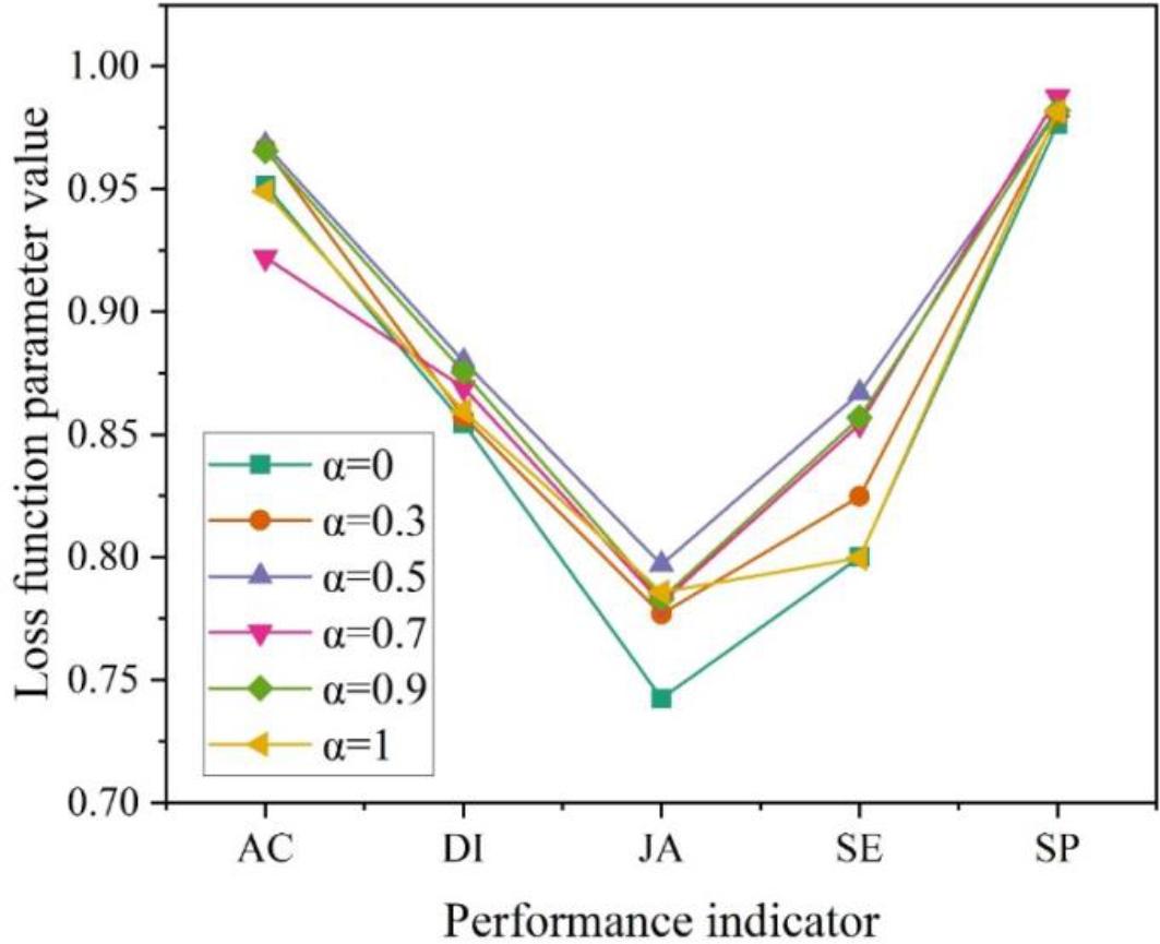
The loss function parameters compare the results of the experiment
In this paper, the proposed TCNet model is evaluated using public image datasets published by ISIC, which are ISIC 2017 dataset, PH2 dataset and ISIC 2018 dataset.
The ISIC 2017 dataset contains 800 skin lesion images for training and 350 skin lesion images for validation.
The PH2 dataset contains a total of 220 skin lesion images. In this paper, the ISIC 2017 training set is used to train the model and the PH2 dataset is used to test the model.
The ISIC 2018 dataset contains 2500 skin lesion images for training. Since the public test set has not been released yet, this paper validates the model performance using cross-validation for a fair comparison.
In this paper, the format, label type, and data division of these three datasets are described in the table. The dataset information is shown in Table 2.
Data set information
| Name | Format | Label type | Training | Data partitioning validation | Testing |
|---|---|---|---|---|---|
| ISIC 2017 | 800 | 350 | 0 | ||
| PH2 | jpg | Pixel level | 0 | 0 | 220 |
| ISIC 2018 | 1865 | 635 | 0 |
The attention mechanism is widely used as an important network optimization module in medical image segmentation tasks, which can improve the network’s ability to learn features in regions of interest. In this paper, we investigate the effect of adding the attention module at different locations in the TCNet network in order to further improve the performance of the network.
Hybrid Attention Module is an attention mechanism module that contains both channel attention and spatial attention. The channel attention mechanism is used to adjust the weights between different channels in the feature map to enhance the weights of useful features. The spatial attention mechanism is used to adjust the weight of each pixel in the feature map to suppress features that are not related to the target region. The hybrid attention module can effectively improve the feature learning ability of the network and the sensitivity of the pixels in the region of interest, thus improving the segmentation performance of the network. In the experiments, the hybrid attention module is added to different positions of the TCNet network, including each basic convolutional unit of the encoder and decoder, cross-layer connection, and up-sampling module, respectively. The experimental results show that the segmentation performance of the network is all improved to some extent after adding the attention module.
This chapter further analyzes the effect of adding the hybrid attention module to the network for segmenting different classes of pixels. The training curves for different joining strategies are shown in Fig. 2. When adding the three attention mechanisms of all-convolution Attention, input-single-output Attention, and input-four-output Attention respectively, it can be found that there are large differences in the fluctuations of the training curves of the three attention mechanisms. The TCNet curve with input four output Attention has a loss value of 0.5 after 1000 times of training, and after 2500 times of training, the training curve tends to flatten out, but the pixel segmentation effect of the overall training curve is more general.
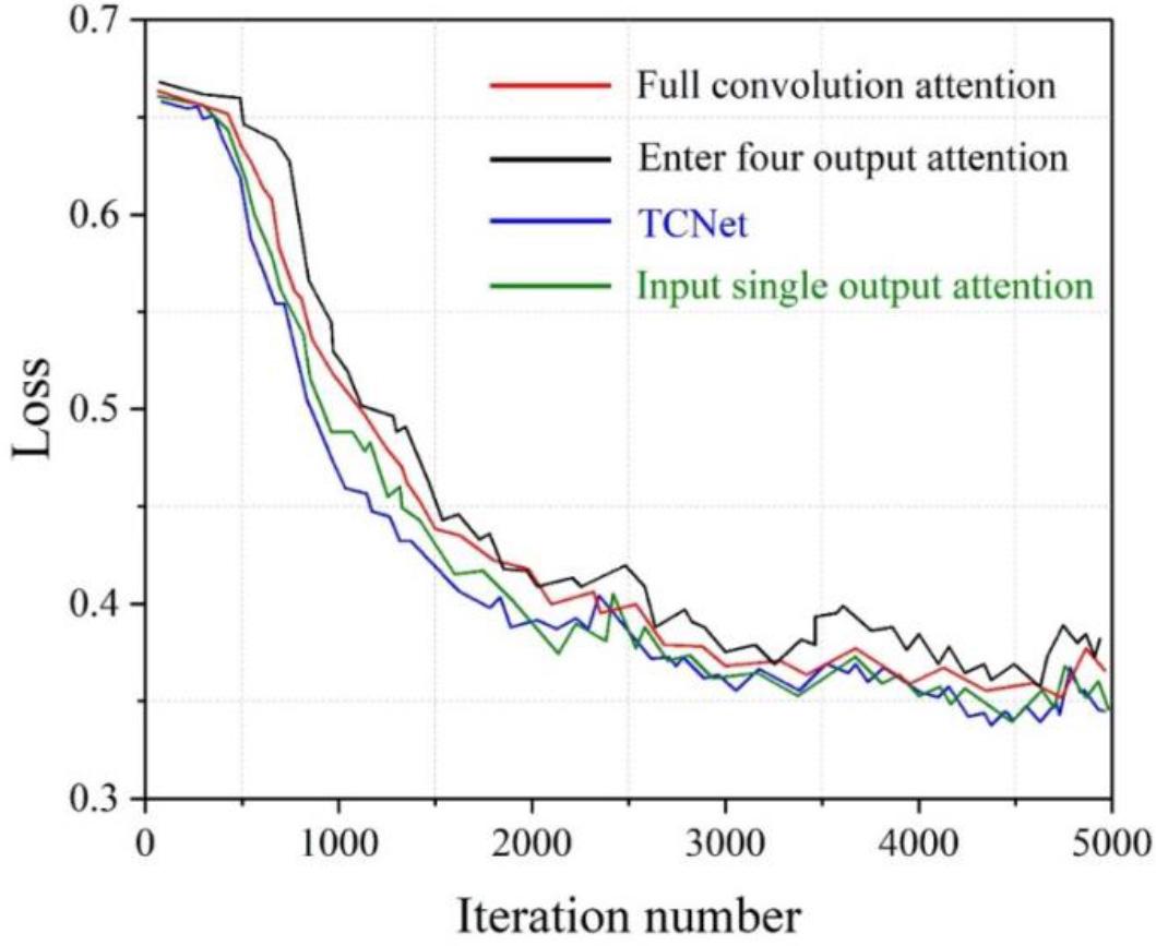
Training curves of different addition strategies
The loss curves of different joining strategies on the test set are shown in Figure 3. After experimental comparison, it can be clearly seen that different strategies for joining the attention mechanism have a huge impact on the performance of the algorithm. From the comparison results in the figure, all the convolutional units are added to the attention mechanism with the best effect. In addition, it is also found in the experimental process that canceling the deep supervision mechanism of TCNet will improve the segmentation performance of the algorithm to a certain extent, and the reason is analyzed to be related to the characteristics of the medical image dataset.
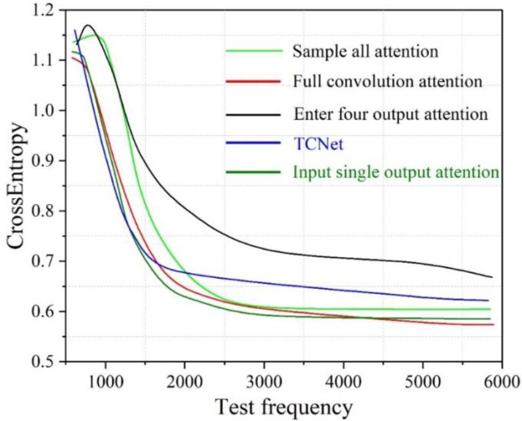
The loss curve of the different addition strategies on the test' set
In order to verify the segmentation performance of the TCNet model, this paper analyzes the model in comparison with advanced segmentation methods. These methods include FCN, UNet, ISL-MSCA, SSLS, mFCN-PI, SBPSF and UNet3+.
Segmentation results obtained by TCNet model and other methods trained on ISIC 2017 dataset and tested on PH2 dataset. The segmentation performance of each model on the PH2 test set is shown in Fig. 4. The TCNet model outperforms the other compared methods in all three metrics, JA, pixel-AC, and DI. Compared with the UNet method, the TCNet model is 2.475% and 3.96% higher in both JA and DI metrics. And compared with SSLS method, TCNet model has significantly improved in pixel-AC index, and the difference between the two in pixel-AC index reaches 11.153%.
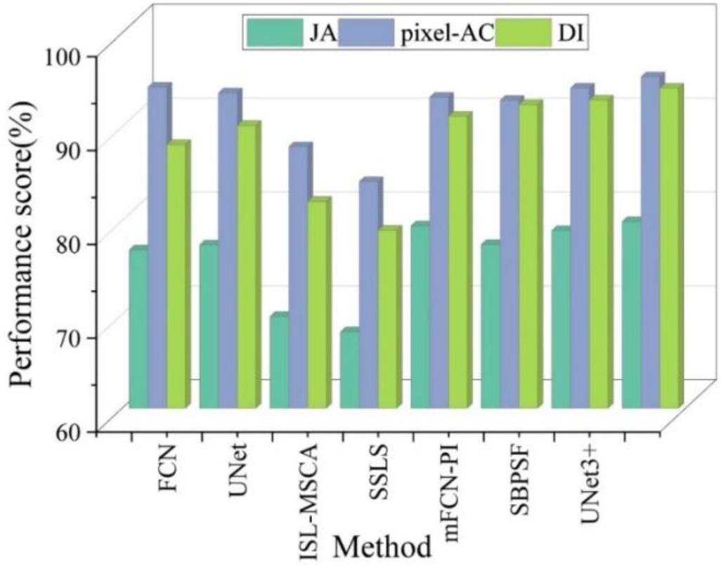
The segmentation performance of each model on the PH2 test set
The segmentation results obtained after cross-validation of the model and other methods on the dataset ISIC 2018 are shown in Figure 5.
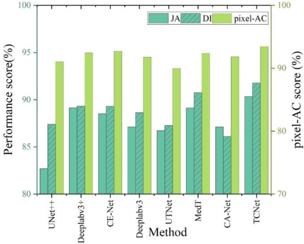
Segmentation performance in the ISIC 2018 validation set
The TCNet model was experimentally compared with several state-of-the-art segmentation networks on the ISIC 2018 dataset, which include UNet++, Deeplabv3+, CE-Net, Deeplabv3, UTNet, MedT, and CA-Net.
UTNet, MedT and CA-Net and TCNet models all use the attention mechanism, the difference is that the TCNet model achieves the extraction of global contextual information and local detail information of the image by using multiple attention mechanisms. The TCNet model proposed in this paper achieves 90.334% JA, which realizes a performance improvement of 7.64% compared to the UNet++ method. On the remaining two indexes, the pixel-AC method and the DI method outperform the other methods, with performance indices of 93.457% and 91.773%, respectively, indicating that the model has a better segmentation performance.
In order to explore and analyze the effectiveness of the TCNet model in segmentation tasks, this chapter conducts ablation experiments on the Large Convolutional Kernel Module (LKM), the Enhanced Transformer Module (ETM), and the Multiscale Feature Fusion Module (MFM) in the decoder. Ablation experiments were performed on two classical datasets.
The DRIVE data were obtained from the Diabetic Retina Screening Program in the Netherlands. It is a classical dataset for evaluating retinal vessel segmentation methods.
The CHASEDB dataset contains 28 retinal images captured from the right and left eyes of 14 school-aged children.
The results of the ablation study on DRIVE and CHASEDB datasets are shown in Table 3. After adding Enhanced Transformer Module (ETM) and Multi-scale Feature Fusion Module (MFM) module to the Large Convolutional Kernel Module (LKM), this image segmentation framework improves the Acc, Sp, and AUC performance indices on the DRIVE dataset. Also on CHASEDB dataset, the increase in Acc, Sen, Sp, and AUC after the addition of LKM module, ETM module, and MFM module in the decoder indicates that the method successfully captures more contextual and advanced information.
Ablation research results in DRIVE and the CHASEDB data set
| LKM | ETM | MFM | DRIVE | CHASEDB | ||||||
|---|---|---|---|---|---|---|---|---|---|---|
| Acc | Sen | Sp | AUC | Acc | Sen | Sp | AUC | |||
| ✓ | 0.925 | 0.836 | 0.972 | 0.966 | 0.958 | 0.875 | 0.975 | 0.982 | ||
| ✓ | ✓ | 0.964 | 0.841 | 0.966 | 0.973 | 0.944 | 0.869 | 0.963 | 0.991 | |
| ✓ | ✓ | 0.952 | 0.869 | 0.979 | 0.987 | 0.957 | 0.873 | 0.967 | 0.985 | |
| ✓ | ✓ | ✓ | 0.973 | 0.824 | 0.983 | 0.989 | 0.970 | 0.889 | 0.986 | 0.992 |
This paper explores the processing performance of an image segmentation algorithm that incorporates an attention mechanism in a deep learning framework. A large convolutional kernel and attention mechanism feature fusion network (TCNet) is constructed, and extensive test experiments of this method are conducted on multiple datasets, and multiple metrics verify the applicability of the method.
In the loss function test of the algorithm, five parameters, accuracy (AC), sensitivity (SE), specificity (SP), Jaccard’s coefficient (JA), and Dice’s coefficient (DI), are used for comparison. Combining the data in the figure, the TCNet method obtains the best performance when the loss function is 0.5. Substituting different hybrid attention mechanisms, the best results are obtained when all convolutional units are added to the attention mechanism. In the classical dataset of medical images, the method TCNet in this paper achieves better performance. And the results of the ablation study on DRIVE and CHASEDB datasets show that the LKM module, ETM module, and MFM module designed in the encoder of this paper can effectively improve the Acc, Sen, Sp, and AUC index values of the image segmentation model. It shows the reasonableness of constructing the large convolutional kernel and attention mechanism feature fusion network in this paper. Compared with the traditional image segmentation algorithm, this method has better performance in segmentation effect and stronger generalization ability.