Research on the Utilization Pattern Mining and Impact Mechanism of Open Government Data Based on Deep Learning Algorithms

Online veröffentlicht: 17. März 2025
Eingereicht: 04. Nov. 2024
Akzeptiert: 13. Feb. 2025
DOI: https://doi.org/10.2478/amns-2025-0183
Schlüsselwörter
© 2025 Ying Zhang et al., published by Sciendo
This work is licensed under the Creative Commons Attribution 4.0 International License.
In the era of digitalization, data has become an important resource for promoting economic and social development. In order to support public monitoring and enhance data reuse in the public sector, more and more government and public sector organizations rely on their open data platforms to disclose information about data in government, science, and other fields and unify the data in the form of datasets posted on the Web [1-2]. The openness and sharing of data is continuously improving the effectiveness of government governance and the quality of public services, and is also a prerequisite for the modernization of the national governance system in the era of big data [3-5].
With the increase in the total number of open government data platforms, there are higher requirements for comprehensive and accurate search and recommendation of open data sets. This is from an overall perspective, as a national-level unified open data platform has not yet been built, datasets are still scattered on top of provincial and municipal platforms, and there is a lack of unified search tools for open datasets, which leads to the inability of data users to realize cross-platform, cross-level, and cross-departmental searches of open datasets [6-9]. In terms of details, although most local government open data platforms provide data users with open dataset search functions based on faceted search and keyword matching, the existing open dataset faceted search systems provided by different platforms differ in the division of domains, departments, etc., which makes it difficult to realize the alignment and aggregation of open datasets from different platforms [10-14].
Nowadays, the new generation of information search and recommendation technologies, such as deep learning, has become a new trend in information acquisition and dissemination and is also the basic content and core task of the national big data strategy [15]. Deep learning techniques can automatically extract semantic information by learning the features and representations of input data and have been widely used in natural language processing, recommender systems, and other fields [16-19]. Its application in open dataset search and recommendation can enhance the discoverability, accessibility and reusability of open datasets, optimize the search and recommendation performance of datasets, and satisfy the user’s demand for efficient, accurate and intelligent search and recommendation of open datasets [20-22].
Based on the content of the ecosystem theory, the study combs through the subjects and connecting links of open government data utilisation, builds an analytical framework for open government data utilisation, and summarises the open government data utilisation model. As an example, open government data is used to analyze and predict traffic accidents, and a prediction model is constructed using deep learning algorithms. Specifically, after building the traffic road network structure, the spatio-temporal features of the accident are captured using the gated graph convolution module, and the attention mechanism is applied to obtain the dynamic weight expression of spatio-temporal. Meanwhile, in order to solve the data sparsity problem and spatial heterogeneity problem of accident prediction, the scale reduction module is introduced to guide the accident risk prediction at the road segment level using the accident risk of coarse-grained regions. Traffic flow data, traffic accident data and weather data from a city’s open government data are used as the dataset for model comparison analysis and case study to explore the model’s prediction performance on traffic accidents and the influence of different features on its prediction error. Then, based on the AMO-TPB theory, the research model of open government data utilisation is constructed, the causes are clarified through regression analysis, and the paths of causes are determined based on the explanatory structural model so as to obtain the influencing mechanism of open government data utilisation.
In the era of the digital economy, data has been formally included in the category of factors of production and plays an increasingly important role in enabling high-quality development of the economy, promoting the transformation of the mode of national governance, and facilitating the change of social lifestyles. The information and data resources in the hands of government departments contain enormous political, economic, and social values. Combined with the basic content of innovation ecosystem theory, we design an ecosystem analysis framework for open government data (OGD) and explore the utilisation patterns of OGD.
The OGD ecosystem analysis framework is shown in Figure 1. This analysis framework is mainly composed of ecosystem subjects and external environment, with openers, developers, and consumers as ecosystem subjects, and the subjects are connected with data chains, achieve interaction and feedback through open platforms, realise data utilisation and value creation and are affected by the economic, social and technological environments.
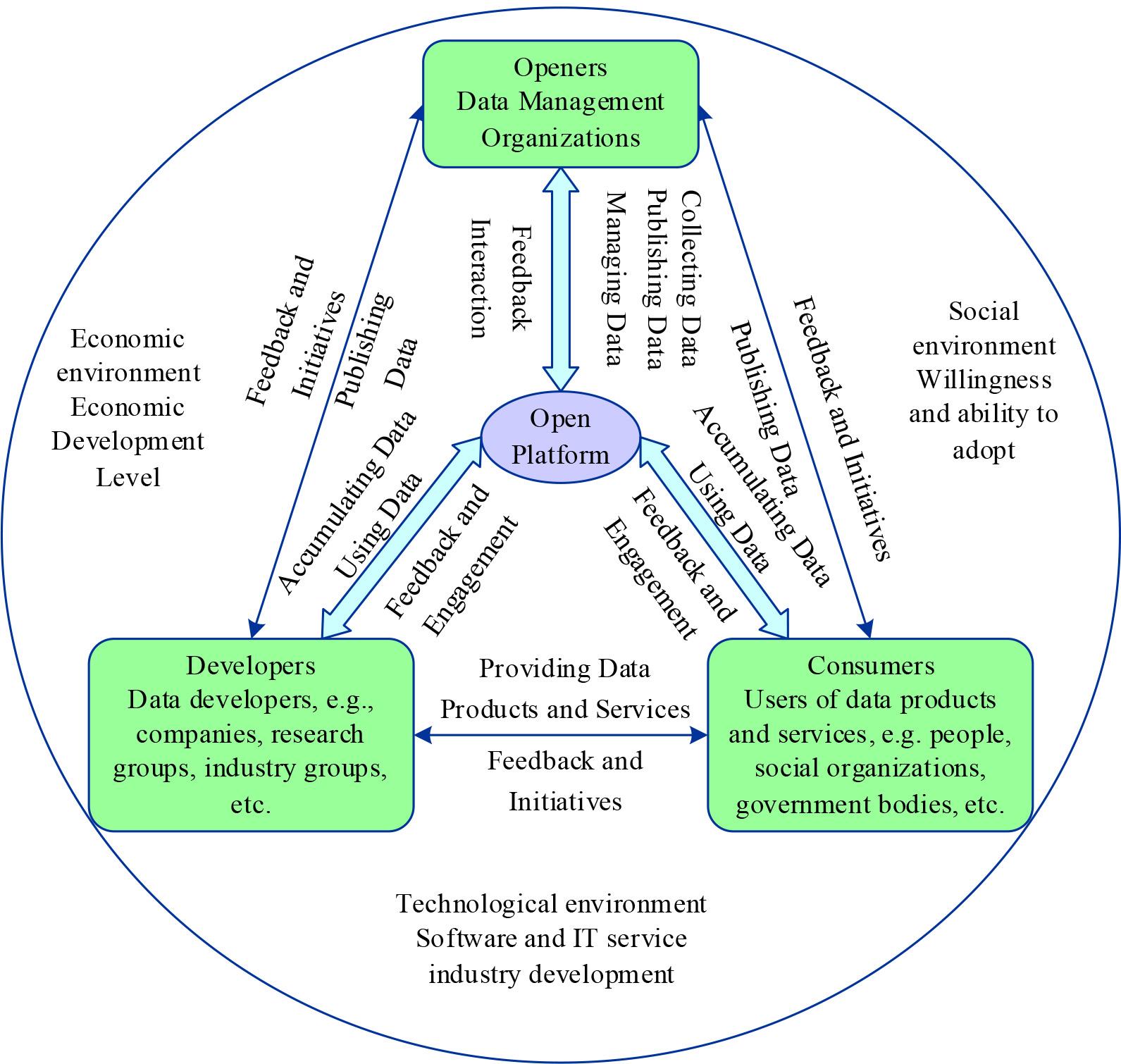
Open government data ecosystem analysis framework
Openers are OGD management organizations, mainly government departments in China, which are responsible for data collection, release, and management. Established studies show that the organisational level of openers, their ability to set standards, policies and regulations, etc., have a significant impact on the level of OGD utilisation. The stronger the openness ability of data providers, the more they can provide huge amounts of high-quality data, thus creating a good foundation for data utilization.
Developers refer to the developers of OGDs, such as enterprises, scientific research groups, industry groups, etc. They are one of the main bodies of data demand and use OGDs to develop data products and services, which promote the utilisation of OGDs and at the same time, serve as a bridge between openers and consumers. The stronger the developer’s data development capability, the more they can explore the value contained in OGD and provide rich and high-quality data products and services, thus enhancing the level of OGD utilisation.
Consumers are the end-users of OGD products and services, which mainly include the public, social groups, and the government itself.OGD can benefit from data products and services, but consumers are also a significant source of feedback and data.Consumers’ ability to consume data products and services influences whether OGD can ultimately realize value-added utilisation.
Open platforms refer to OGD portals, which are data carriers and interaction channels, mainly online platforms, such as the OGD platforms built by Chinese provincial and municipal governments.The OGD ecosystem’s various subjects are connected through the open platform.
In the OGD ecosystem, data are integrated into the open platform and flow between the various ecosystem subjects throughout the whole process, from openness to value creation to data return, forming a data chain connecting the whole ecosystem. Specifically, data is initially released and managed by openers through the open platform, then flows to developers and is processed into corresponding data products and data services, and then flows to consumers to realise value creation in corresponding scenarios. Accompanied by the feedback and interaction between the actors in the OGD ecosystem, the flow process of each link also creates and accumulates new data, and the new data becomes the object of the next round of data opening to realise the return flow and cycle.
Different government open data utilisation models can be divided into government-led open data utilisation models, enterprise-led open data utilisation models, and citizen-led open data utilisation models.
Government-led open data utilisation models can be divided into internal management utilisation models, social innovation application models, and commercial development co-creation models according to different value objectives.Enterprise-led open data utilisation models can be divided into product co-creation models, service co-creation models, and knowledge co-creation models.A citizen-led Open Data Utilisation Mode is the practice of diversified exploitation of government open data by individual citizens or citizen groups in collaboration with different stakeholders based on their or common interests.
Specifically, for example, in the internal management utilisation model, a municipal government needs to set up a city operation monitoring system for dynamic monitoring in order to achieve comprehensive management, command, decision-making and scheduling of the city. Although different government departments have opened up data reflecting the city’s situation, including traffic flow, population flow, public security, water, electricity and gas situation, etc., there is a lack of unified development and utilisation planning methodology and realisation technology. In order to realise the value of these open data, the municipal government takes the lead and provides financial and policy support, and sets up a data studio to research and put forward demands, and cooperates with data companies, internet enterprises, application developers to carry out open data-based development and utilisation. Developers are implementing a project to develop a city operation monitoring system based on open data. In this process, open data can be analysed using data mining and deep learning algorithms, resulting in the data products needed by the government, which can assist the government’s urban management agencies in conducting real-time remote monitoring of the city’s operation and provide accurate data support for decision-making. The following is an example of traffic accident risk prediction in the city, using deep learning algorithms to construct a risk prediction model for analysis, and mining the internal management and utilisation model of open government data.
This chapter proposes a scale-reduced attention and graph convolution-based prediction model (SAGCN) using open government data to divide urban areas into road segments.
The details of the model for the accident risk prediction part are shown in Fig. 2, where the historical long-term and short-term accident risks are fed into the gated graph convolution unit separately, and the weather features of the corresponding time slices are fused in its output results, and finally, the splicing is done. The attention mechanism is used in the time layer, and this result and the coarse-grained accident risk are fed into the feature layer, and the output result of the scale reduction module is fused with the output result of the feature layer.
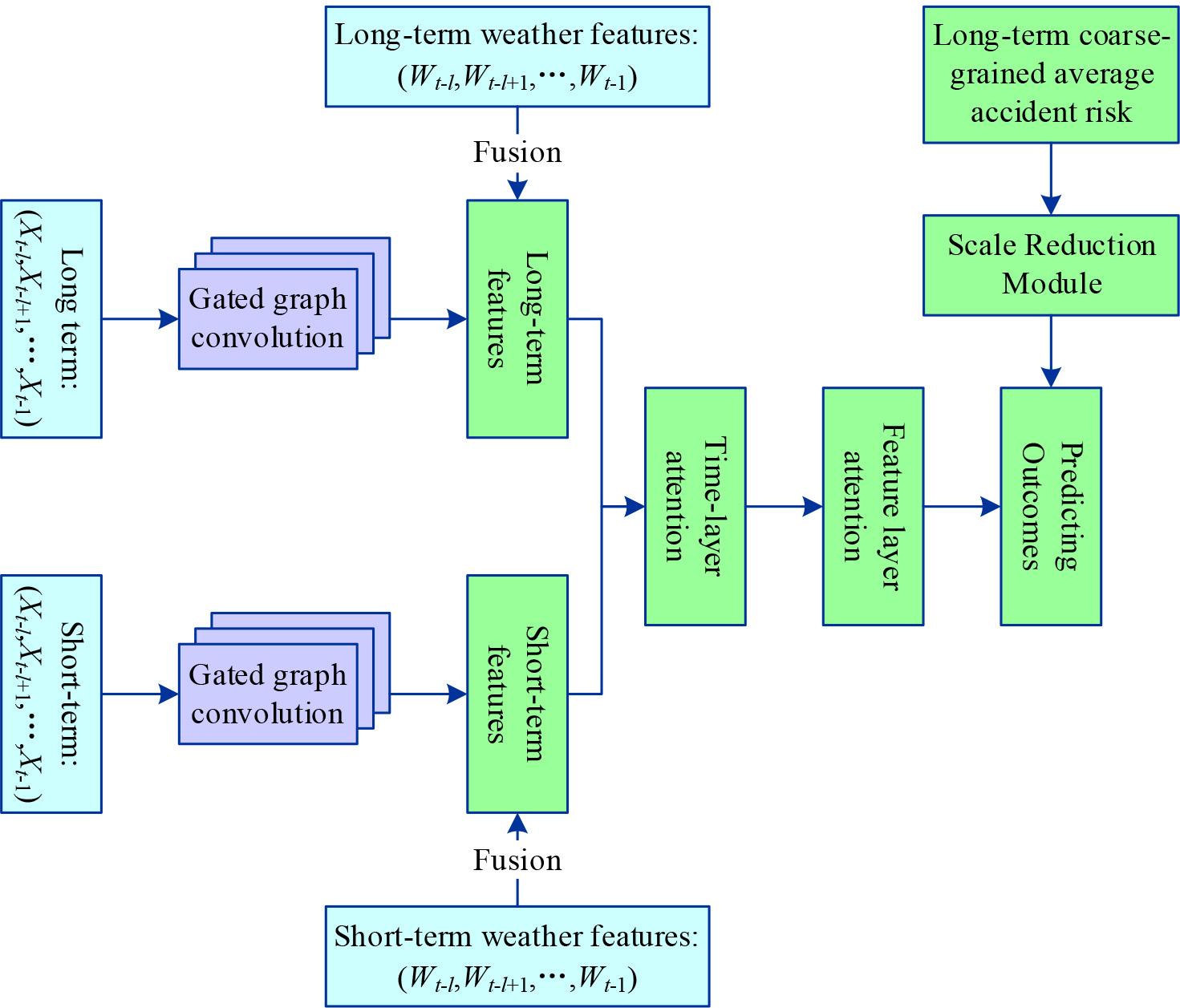
Details of the model of the accident risk prediction
The gated graph convolution module allows for the simultaneous extraction of spatio-temporal features. For the historical long-term input, the input
The implementation of GCN is based on spectral graph theory: given an abstract graph
As shown in Eq. (2), according to the convolution theorem, the signal
Given the complexity of the eigenvalue decomposition of the Laplace matrix,
In order to model the non-linear spatio-temporal correlations in accident prediction, the final outputs use gated linear unit activation outputs as shown in Eq. (4), which selects the partial information in the linear variations by multiplying the linear transformations with the non-linear activations:
Where
The long-term features obtained by the gated graph convolution unit and their corresponding normalised weather features (
Input the temporal feature
Where
The above equation notation is to illustrate the dimension size of each parameter.
The output of the temporal layer attention mechanism is accumulated from the time score results of each step, which are calculated as follows:
Where
In the result
Where
The preliminary results obtained from the final feature layer are shown in Eq. (14), where
Due to the large number of accident risk values in the sample that are zero, normal outputs will tend to predict all-zero values in order to reduce the error, a phenomenon known as the zero-inflation problem. In order to solve this problem, the scale reduction module is designed in this paper to combine the above results with the output.
The Scale Reduction Module takes as input accident risk values in coarse-grained areas with large spatial scales. The structure of this module is a three-layer feed-forward fully connected layer. The input layer of the triage module is denoted by
In this experimental design, the massive urban traffic accident data open to the government are fused with multi-source data such as real-time traffic flow and weather, and the effects of multi-source input data and single-source traffic flow data on the risk of traffic accidents occurring in the relevant area are calculated separately, in order to find out and compare the extent of the effects of various models and different input data on the risk of traffic accidents.
The datasets used in this paper include three: traffic flow data, traffic accident data and weather data (rainfall and visibility). It is collected from open government data from June to December 2022 of a city. The processed raw dataset is split into training data, validation data and test data according to the ratio of 7:1:2, which is used for model training and validation.
In the experiments of this paper, the error functions of mean absolute error (MAE), mean squared error (MSE) and mean relative error (MRE) are used as the evaluation indexes of the algorithm. The smaller the value of the above three evaluation indexes, the more accurate the prediction results will be. This experiment predicts the risk of traffic accidents in the grid area, and the range of the predicted value is located between 0 and 1. When the predicted value is closer to 1, it means that the probability of traffic accidents in the area in the next time interval is greater.
This paper employs Linear Regression (LinR), Logistic Regression (LogR), Decision Tree (DT), Random Forest (RF), Support Vector Machine (SVM), and Stack Noise Reduction Autocoding (SDAE to compare various algorithms.
The comparison of the experimental results of different models in the case where the input source is only traffic flow is shown in Figure 3. It can be found that (1) the prediction accuracy of deep learning models is overall higher than that of machine learning models. The reason for this is that the deep learning model is better at learning high-dimensional features and has a stronger learning ability than the machine learning model. (2) The prediction error of the SAGCN algorithm proposed in this paper is smaller than that of the SDAE model, and the values of its MAE, MSE, and MRE are 0.082, 0.038, and 0.808, respectively.
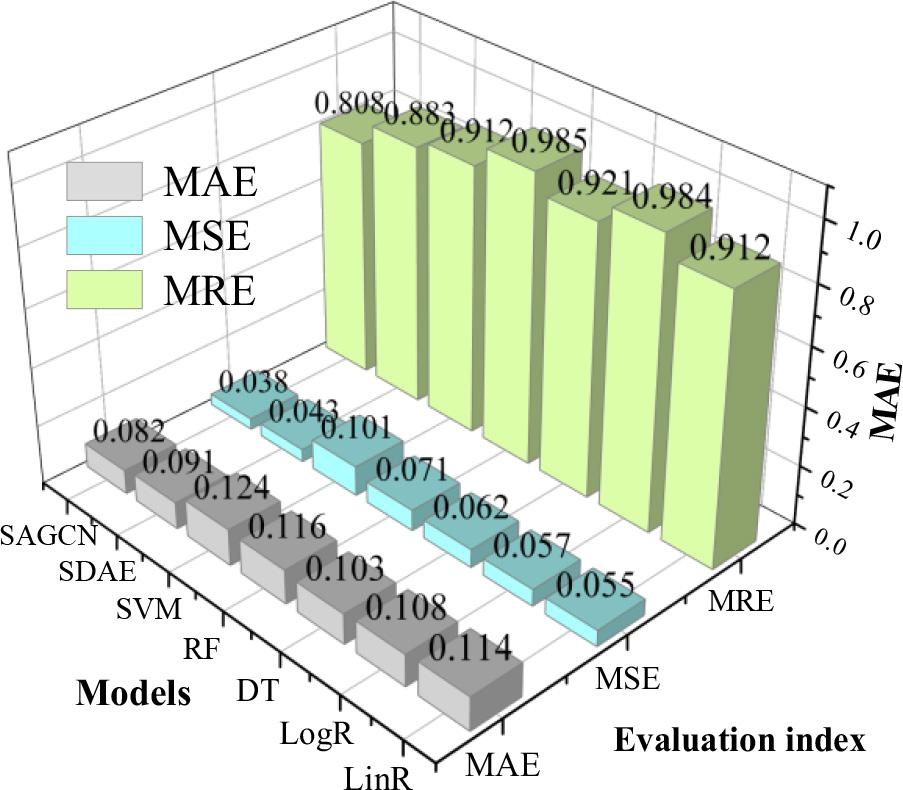
Comparison of experimental results of different models
The proposed SAGCN model is combined with dynamic factors such as traffic accident data and weather data to carry out large-scale experiments to compare the impact of different influencing factors on the prediction of traffic accident risk in a city urban area.
A comparison of the experimental results based on various factors is shown in Table 1, where F-flow rate, A-number of traffic accidents, R-rainfall, and V-visibility are shown. The errors of the combination of flow, the number of historical accidents, rainfall and visibility are not the smallest, and the combination model of flow, the number of historical accidents, and rainfall has the smallest overall error, with MAE, MSE, and MRE of 0.075, 0.035, and 0.756, respectively, while the combination model of flow, visibility and rainfall has the largest error, with MAE, MSE, and MRE of 0.085, 0.044, and 0.851.
| Input dimension | MAE | MSE | MRE |
|---|---|---|---|
| SAGCN(F) | 0.081 | 0.041 | 0.784 |
| SAGCN(F+A) | 0.077 | 0.039 | 0.776 |
| SAGCN(F+R) | 0.078 | 0.040 | 0.768 |
| SAGCN(F+V) | 0.083 | 0.038 | 0.836 |
| SAGCN(F+A+R) | 0.075 | 0.035 | 0.756 |
| SAGCN(F+A+V) | 0.083 | 0.038 | 0.836 |
| SAGCN(F+R+V) | 0.085 | 0.044 | 0.851 |
| SAGCN(F+A+R+V) | 0.082 | 0.042 | 0.844 |
Considering single factors other than traffic flow, factors such as the number of historical accidents and rainfall are beneficial in reducing the error of the experimental results, while the visibility factor leads to an increase in the error of the experimental results. Therefore, it is not the case that the more combinations of factors are considered, the more favourable it is to reduce the prediction error of the model, and there are differences in the results of different combinations of factors. In this paper, rainfall and the number of accidents are favorable factors for reducing the prediction error of the risk of traffic accidents in the experiments.
Since different causal factors have different impacts in different scenarios, this section conducts model training for different scenarios, such as morning peak and flat peak, weekdays and holidays, and sunny and rainy days, in that order.
The comparison of the experimental results (MRE) for the morning peak and the flat peak is shown in Figure 4. The MRE of the prediction results for the morning peak is between 0.734 and 0.798, which are all lower than that of the flat peak.The prediction errors of various factors on the risk of traffic accidents are generally in line with those in the utility analysis mentioned earlier. There are more vehicles on the road during the morning peak.If a road traffic accident occurs, traffic congestion will be more serious than in the flat peak. Therefore, it is particularly important to accurately predict the risk of traffic accidents during the morning peak. The prediction errors of this paper’s model on the risk of traffic accidents in the morning peak are lower than those in the flat peak, which can help the personnel of the traffic management department to deploy the police to the high-risk areas of accidents in the morning peak in advance, and deal with the accidents in a timely manner, and can also help the drivers to avoid high-risk areas.
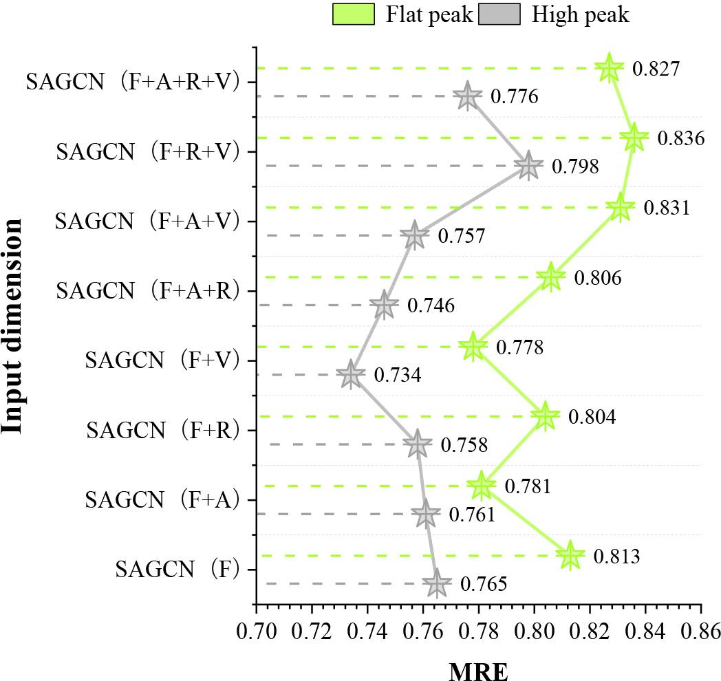
The experimental comparison results of high peak and flat peak(MRE)
The effect of each different input on the model prediction error for weekdays and holidays was compared, and the comparison of the experimental results (MRE) for weekdays and holidays is shown in Figure 5. The model prediction MRE values for weekdays and holidays are 0.736~0.813 and 0.769~0.839, respectively. There are more vehicles on weekdays, and traffic congestion caused by road traffic accidents is more serious than that on ordinary holidays, so effective prediction of the risk of traffic accidents on weekdays is particularly important, and the prediction errors of this paper’s model on weekdays are lower than that of holidays, which can help the public to plan their routes to avoid high-risk areas. Citizens travelling on weekdays should plan their routes to avoid high-risk areas.
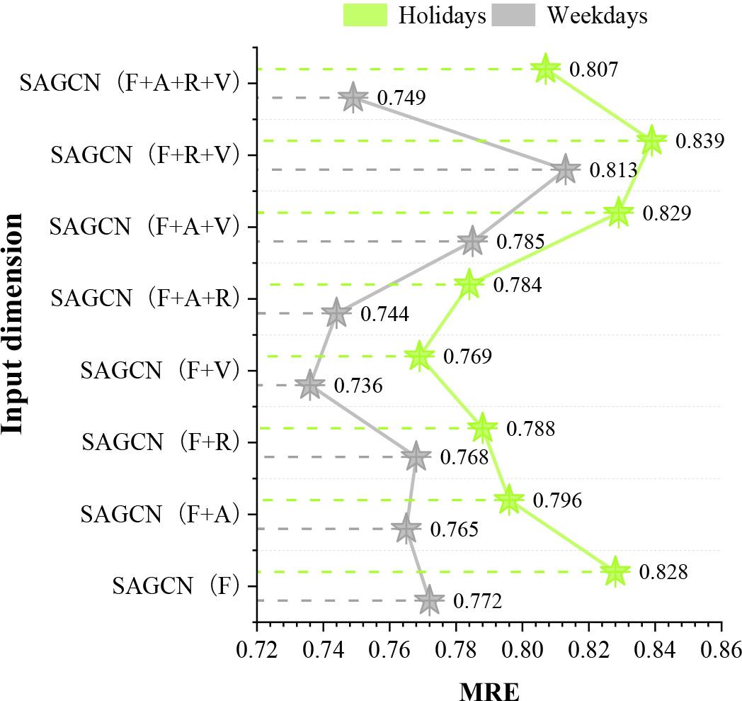
The experimental comparison results of weekdays and holidays(MRE)
The comparison of experimental results (MRE) between sunny and rainy days is shown in Figure 6. The model will show slightly better prediction results on rainy days than on sunny days, and the MRE for the prediction of traffic accident risk on rainy days is 0.745~0.781, and the MRE on sunny days is 0.772~0.793.
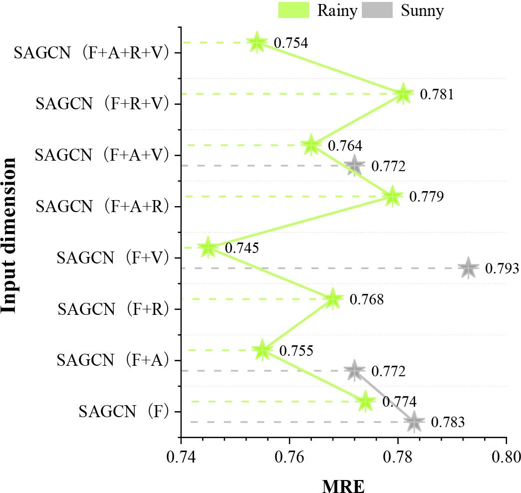
The experimental comparison results of sunny and rainy(MRE)
In summary, open government data such as traffic flow, weather data and traffic accident data can be used to predict the risk of traffic accidents using deep learning models to help the relevant personnel make decisions and plans to reduce the occurrence of traffic accident incidents.
Open government data itself does not bring economic value and social benefits, but the public, as developers and utilisers of data, can provide valuable information and collective wisdom to create economic value for society, and public participation largely influences the value realisation of government data. After applying deep learning algorithms to deduce the process of open government data utilisation, this chapter explores the influence mechanism of open government data utilisation based on the perspective of the paradox of public utilisation willingness and behaviour, combined with regression analysis.
The main object of regression analysis is the statistical relationship between the variables of objective things, which is based on a large number of experiments and observations of objective things and is used to find the statistical regularity hidden in those phenomena that seem to be uncertain. Examining the interdependence of one variable (the dependent variable) with many other variables (the independent variables) is a multiple regression problem.
Once a multiple regression model has been determined, it is obviously not prudent to apply the model immediately for prediction, control and analysis, because whether the model reveals the relationship between the explanatory variables and the explanatory variables must be determined by testing the model. The testing of regression models generally requires the use of statistical tests.
Statistical tests are usually tests of the significance of the regression equation and the regression coefficients, as well as tests of goodness-of-fit and multicollinearity of the explanatory variables.
Let the linear regression model of random variable
Where
For a practical problem, if
Where
Goodness of fit is used to test the fit of the regression equation to the sample observations, as reflected in the value of the sample coefficient of determination
The sum of squares decomposition formula is:
The regression sum of squares,
The residual sum of squares
The total sum of squared deviations
From the significance of the regression sum of squares and the residual sum of squares, it can be known that the greater the proportion of the regression sum of squares in the total sum of squares of deviations, the better the linear regression, which indicates that the regression straight line fits the sample observations better, and if the proportion of the residual sum of squares is large, the regression straight line does not fit the sample observations satisfactorily. The ratio of the sum of squared regressions SSR to the sum of squared total deviations SST is defined as the coefficient of determination:
The coefficient of determination
Effect of multicollinearity on regression models
Set up the regression model:
There exists complete multicollinearity, i.e., for the column vectors of the design matrix
The rank
2) Diagnosis of multicollinearity
Centre normalising the independent variables, then
Since
AMO theory is the ‘ability-motivation-opportunity’ theory, which believes that an individual’s ability, motivation and opportunity together determine their behavioural tendencies, while TPB theory (Theory of Planned Behaviour) believes that perceived behavioural control, behavioural attitudes and subjective norms together influence the emergence of behaviours. Combining AMO-TPB theory, this paper constructs the theoretical framework of AMO-TPB.
The research model of open government data utilisation is shown in Figure 7. The capability dimension contains perceived behavioural control and data literacy, i.e., the degree of control felt by the public when using government data and the public’s data awareness and capability. The motivation dimension contains behavioural attitudes and subjective norms, i.e., the public’s evaluation of the behaviour of utilising government data and the social pressure felt by the public to perform the utilisation behaviour. The opportunity dimension includes facility readiness, data quality and platform quality, i.e., the readiness of the infrastructure that the public has to support the utilisation behaviour, and the availability and ease of use of government data and open government data platforms. In addition, individual characteristics such as gender and age affect the consistency between individual willingness and actual behavior. Risk attitude is the individual’s tendency to choose between risky and safe options. In this paper, risk attitude refers to the public’s weighing and choosing between risky and safe options when facing whether to make use of government data or not, and it is also an important factor that affects the relationship between individual willingness and actual behaviour. Therefore, this paper argues that gender, age, and risk-taking attitude also have an impact.
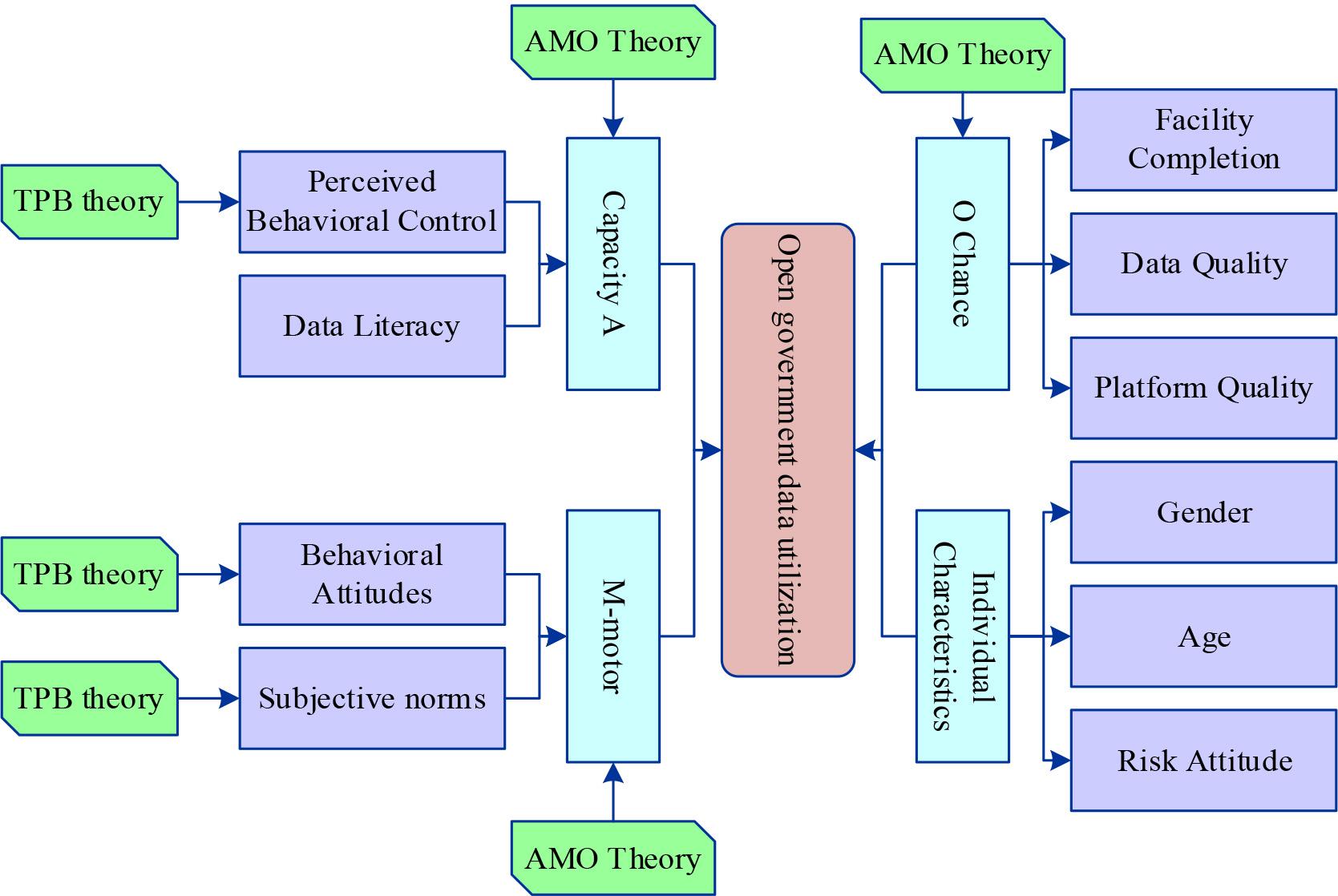
Open government data utilization model
The independent variables in this paper are 10 variables that fall under the dimensions of ability, motivation, opportunity, and individual characteristics, and the dependent variable is the utilization of open government data. Considering that the research object is the general public, the questionnaire needs to be widely applicable, so the questions are set in accordance with the principle of simplicity and comprehensibility. The total number of questionnaires returned was 525, with 483 of them being valid, with a validity rate of 92%.The survey sample is representative of different provinces, age groups, and genders in the PRD region.The collected data passed the reliability and validity tests.
In this paper, the variance inflation factor (VIF) was applied to test the independent variables for multicollinearity. The estimation results of the research model are shown in Table 2. *** denotes p<0.001 and ** denotes p<0.01. The maximum value of VIF for the respective variables is 4.537, and there is no multicollinearity or weak covariance between the variables. The regression model was screened in 7 steps using the backward LR strategy, and the log-likelihood value of -2 times the last step was 309.239, which passed the significance test of the regression equation. The Hosmer-Lemeshow statistic was 0.531, and the model fit was good.
| Variable class | Variable | Regression coefficient | Standard deviation | |
|---|---|---|---|---|
| Ability | Perceptual behavior control | 0.133*** | 0.034 | 0.912 |
| Motive | Behavior attitude | 0.322** | 0.055 | 0.817 |
| Opportunity | Complete facility | 0.208*** | 0.049 | 1.172 |
| Data quality | 0.156*** | 0.124 | 0.924 | |
| Individual characteristics | Risk attitude | 0.695*** | 0.537 | 0.915 |
| Constants | 0.776** | 0.489 | 3.226 | |
| Model(Sig.) | 0.000 | The logarithmic likelihood of the minus double | 309.239 | |
| Hosmer-Lemeshow | 0.531 | |||
Perceived behavioral control has a significant positive effect (0.133) on the utilization of open government data. A high level of perceived behavioural control helps to reduce uncertainty and anxiety during public utilisation of open government data, a finding that reveals the key role of public confidence and sense of self-control in utilisation behaviour. Meanwhile, behavioural attitude (0.322) in motivation, facility completeness (0.208) and data quality (0.156), an opportunity and risk attitude (0.695) in individual characteristics also have a significant positive effect on open government data utilisation. In comparison, other variables did not have a significant effect on the utilization of open government data.Among them, risk attitude in individual characteristics has the greatest effect on the use of open government data.
Perceived behavioral control, behavioral attitudes, facility completeness, data quality, and risk attitudes are denoted by S1, S2, S3, S4, and S5, respectively, and S0 denotes the utilization of open government data. After the element hierarchy analysis through the adjacency multiplication matrix, the influencing factors of open government data utilisation are divided into 2 layers: layer 1 L1 = {S3, S4, S5} and layer 2 L2 = {S1, S2}. According to the factor level situation and the complex interrelationship between the factors, the explanatory structure model is obtained. The explanatory structure model of open government data utilisation is shown in Figure 8. Open government data utilisation includes both shallow and deep factors, which form three paths of action:
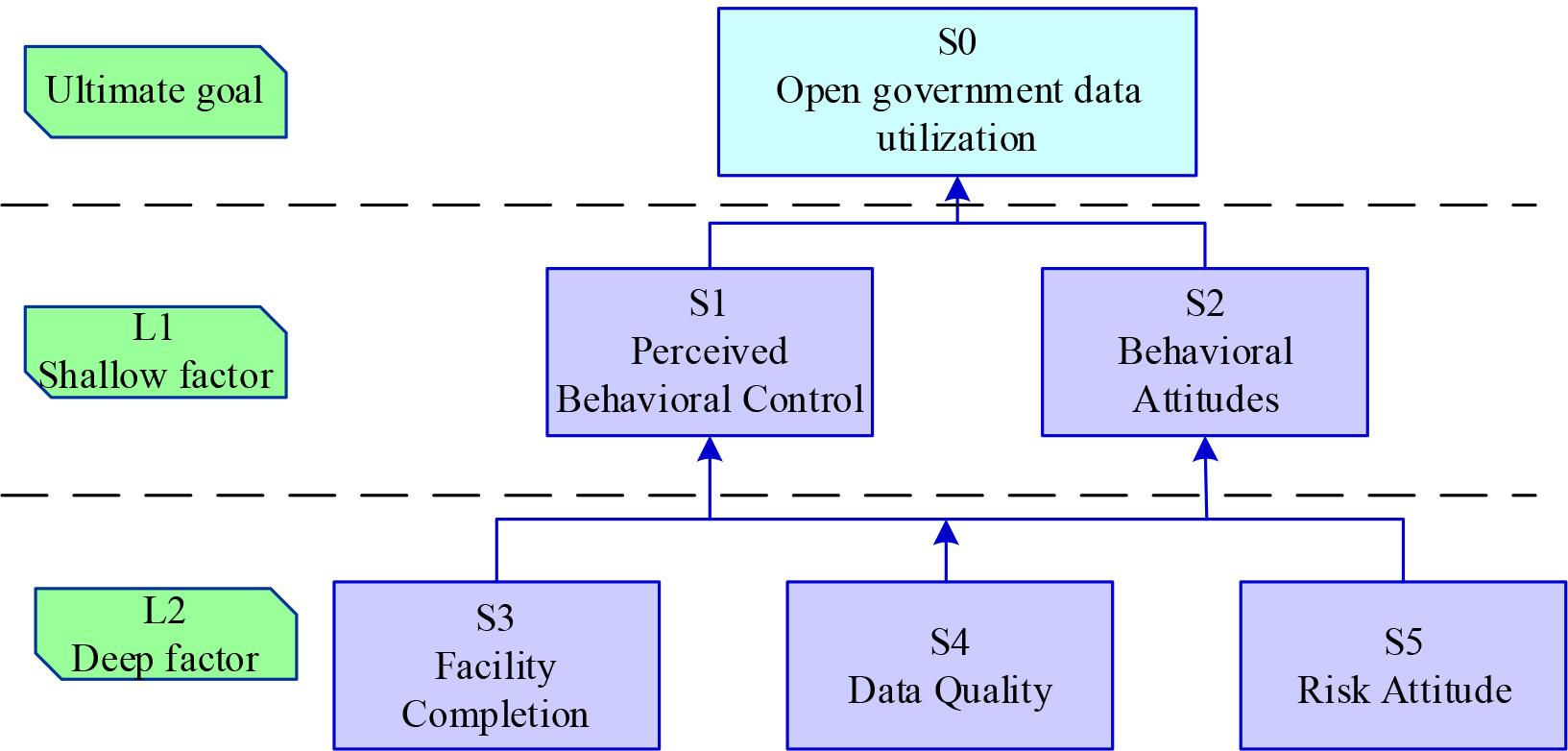
Explaining structural models for open government data use
Path I: Facility Completion → Perceived Behavioural Control / Behavioural Attitude → Open Government Data Utilisation
Path 2: Data quality → perceived behavioural control/behavioural attitude → open government data utilisation
Path 3: Risk Attitude → Perceived Behavioural Control / Behavioural Attitude → Open Government Data Utilisation
Effective utilization of open government data is beneficial for both promoting urban economic development and enhancing public services. In this study, we analyze the open government data utilization model, starting with the government-led internal management utilization model, taking traffic accident risk prediction as an example, constructing an intelligent model based on scale-reduced attention and graph convolution, and conducting experimental analysis. Then, using the regression analysis method, based on the constructed research framework on open government data utilization, the influence mechanism of open government data exploitation is explored.
In traffic accident risk prediction, the MAE (0.082), MSE (0.038), and MRE (0.808) of the SAGCN model in this paper are smaller than those of the comparison models and have better traffic accident prediction performance. For the feature analysis, the number of historical traffic accidents and rainfall help to reduce the prediction error of the model, while the visibility increases the model’s error, which is not conducive to improving the prediction accuracy. In addition, the SAGCN model in this paper has better performance during busy traffic times (morning rush hour, weekdays) and when there is an unusual event (rainfall), corresponding to MREs of 0.734-0.798, 0.736-0.813 and 0.745-0.781. The deep learning model based on open government data can predict the potential risks of traffic, which makes it easier for relevant people to make proper precautionary efforts to reduce casualties and property losses.
Perceived behavioral control, behavioral attitudes, facility completeness, data quality, and risk attitudes all have a significant positive effect on open government data utilization (p<0.01). Risk attitudes among individual characteristics have the most obvious effect on open government data utilization, with a regression coefficient of 0.695. The way that open government data is used is affected by three paths: facility completeness, data quality, and risk attitudes. All three have a significant positive effect on open government data use (p<0.01), with a regression coefficient of 0.695. Perceived behavioral control/behavioral attitude has a facilitating effect, which promotes the utilization of open government data.