Health Management Strategies for Medical Health Records Incorporating Graph Theory Methods

Online veröffentlicht: 17. März 2025
Eingereicht: 29. Okt. 2024
Akzeptiert: 13. Feb. 2025
DOI: https://doi.org/10.2478/amns-2025-0166
Schlüsselwörter
© 2025 Yanjie Wang et al., published by Sciendo
This work is licensed under the Creative Commons Attribution 4.0 International License.
Personal health data integration and circulation is one of the important parts of China’s medical and health system reform. As a promising self-management tool for personal medical and health data, personal health records, together with electronic health records and electronic medical records, constitute the core content of personal health data [1-3]. Health records are important information for recording personal health status, including disease history, family medical history, living habits, and health examination results. In order to better manage personal health information, it is crucial to develop a scientific, rational and systematic health record management strategy [4-7].
Healthcare records are formed by each healthcare organization in the course of medical business activities, and are used to record the process of medical activities, details of medical activities, and the results of medical activities, and contain a large amount of valuable medical information. As a basis for dealing with doctor-patient disputes, medical and health records can provide valuable information for scientific research and education, which is not only an important support for medical services but also an important guarantee for medical quality and safety [8-11]. Therefore, in the information society, it is necessary to carry out the transformation of informationization of medical and health record management. The in-depth promotion of the application of information technology in healthcare records management is necessary for the development of healthcare records management business and the promotion of people’s health quality management [12-14]. At the same time, the network is a double-edged sword. In the process of promoting the construction of medical and health record informatization, the relevant personnel grasp the opportunities brought about by clear information technology, and at the same time, they should also recognize the challenges brought about by the application of information technology in order to continuously improve the construction of information technology in medical and health record management [15-18].
Literature [19] launched a cross-sectional study of hospitals using electronic cases in order to explore the impact of the application of electronic medical records on the quality of healthcare services. The results were analyzed through questionnaires and descriptive and statistical analyses using the Statistical Package for the Social Sciences (SPSS), and the results confirmed that electronic medical records are conducive to improving the quality of healthcare services. Literature [20] reviewed the literature related to “personal health records” in various fields and analyzed the results to show that the phrase is an extension of the electronic record and outlined several aspects of archives and records management that can be effectively studied in personal health records. Literature [21] utilized cross-sectional, descriptive, and comparative design methods to examine the differences in healthcare delivery between hospitals using paper cases and electronic medical records. A comparative test analysis concluded that the adoption of electronic medical records was beneficial in improving the quality of healthcare services. Literature [22] emphasized the important role of “lean management” in hospitals. Interviews and observations were conducted with medical records department personnel and hospital experts. The results of the study indicated that the medical records department is an important part of the hospital’s information system, and it is important to use lean management to improve the daily work of this department. Literature [23] mentions a secure management framework for patient medical records based on Ethernet blockchain to provide correctness in medical records lifecycle management. By utilizing a secret sharing scheme where shares are attributed to the patient, it aims to give individual patients full control over their medical records. Literature [24] evaluated a distributed security module for clinical images by using the RC6 encryption algorithm and CSIS for distributed storage of clinical images and sharing them using a fully secret sharing scheme. It is considered to be able to publicize individual key sharing and “n” image sharing as the scheme has strong, perfect security.
Literature [25] was based on a questionnaire to understand the importance of using electronic medical records for patients. The results of the study showed that electronic medical records not only effectively save healthcare resources, but patients can also realize their health management through electronic medical records. Literature [26] explored the blockchain electronic medical record management framework, which utilizes blockchain technology to ensure the security and privacy of medical information management and realizes the authenticity and integrity of the medical record through records for off-chain storage, and also emphasizes that the patient is the exclusive property of the medical record. Literature [27] proposes a blockchain technology framework for electronic medical record management. The results obtained through proof of concept in medical clinics indicated that private health organizations have relatively low security and efficiency in the management of electronic medical records, and the development of technological solutions for the management of electronic medical records is an effective measure to address this issue. Literature [28] discusses the use of blockchain networks for solving the problems in medical record systems with the aim of enhancing the patient’s control access to the medical records while healthcare professionals need to access and update the medical records with the patient’s permission and authorization to achieve the integrity and security of the medical record data. Literature [29] developed a medical record management framework in order to support healthcare delivery in hospitals. Relevant data from several hospitals were collected through quantitative analysis, questionnaires, etc. The study emphasized the deficiencies in medical record management in public hospitals and developed a framework for improving medical record management.
The study aims to develop a disease prediction model to enhance the effectiveness of healthcare management.In this paper, the DHG4DP model is constructed by extracting the symptom information of patients from the electronic health record (EHR). Then, the large hypergraph is divided into two sub-supergraphs so that DHG4DP can both globally mine the patient-disease relationship and discover specific disease-accompanying patterns. In addition, the model associates the sub-supergraphs with the patient’s time-series information, constructs dynamic sub-supergraphs, and organically integrates the disease relationships extracted from the two dynamic sub-supergraphs with the subdivided disease types, ultimately realizing the improvement of the disease prediction accuracy. The constructed model is practically applied in medical work, and the management effect is examined through controlled experiments.
In traditional medical activities, the diagnosis and treatment of diseases have a certain delay. That is, before the onset of the disease, doctors can not accurately determine whether the patient is sick or not, and it is difficult to realize the dynamic prediction of the patient population. In the new era, artificial intelligence technology has been widely used in the field of medicine, and disease prediction is widely supported by this technology.Dynamically analyze the prevalence of diseases in the population, while also effectively analyzing the social environment, population immunity, and other factors.In addition, with the support of the corresponding mathematical model, it can dynamically predict and analyze disease prevalence, which provides an effective basis for the hospital’s health management strategy.This paper combines the graph theory method with medical and health records to construct a disease prediction network model that promotes medical and health management.
Medical Health Record (EHR) data refers to a longitudinal patient electronic medical information collection system that can record all data generated by a patient at a healthcare facility.EHR contains a wide variety of data and information about a patient, such as patient demographics, medical history, medication and allergy history, immunization status, lab test results, radiological images (e.g., X-rays, etc.), vitals, personal data such as age, height, weight, etc., medical procedure records, payment information, etc. This information plays a vital role in analyzing patient characteristics and helping physicians make decisions. [30].
It is still difficult to directly apply readily available mathematical formulas to computationally analyze a patient’s medical and health records. Instead, some analytical methods in complex networks and graph theory can be employed to map multiple data and information about patients onto the structure of networks and graphs for intuitive visual representation [31]. Quantitative computational analysis is performed through the dynamics of the model to understand and analyze the laws and properties embedded in the EHR.
The use of finite graphs to describe the EHR process uses vertices and undirected edges, which together then form an undirected graph
Therefore, if this undirected graph
In addition, this undirected graph can be represented by another association matrix
At this point, the connection between the behavior and the data is established using some basic methods of graphs.
When there are a total of
So the more edges a vertex
The distribution of degrees describes the conceptual problem of analyzing the complexity of graphs in undirected graphs.
After representing a complex behavior as an undirected graph with
With the development of graph neural networks, dynamic graph neural networks have received attention for their ability to flexibly model temporal information. In addition, multimodal methods also shine in various fields of deep learning. Multimodal can utilize multiple forms of information, and through certain fusion methods, the effect is better than the effect of unimodal methods. [32].
The Dynamic Hypergraph Neural Network based Disease Prediction Model (DHG4DP) designed in this paper is shown in Figure 1. The model first processes the dataset. The symptom information of the patient is extracted first, and this information is used to initialize patient embedding. Then, the model extracts the global disease relationship graph and constructs the local disease hypergraph and sudden disease hypergraph based on this graph.In the second step, the model distinguishes the diseases into persistent and emergent diseases and performs hypergraph convolution and feature fusion on the disease embedding according to the two sub-hypergraphs constructed in the previous step to obtain the disease embedding. In the third step, the model handles the temporal relationship to categorize the impact of the disease on the patient into long-term disease, emergent-associated disease, and emergent-unassociated disease, and then through the attention mechanism to Generate the embedding of each hospitalization record of the patient, and then model the temporal information of the patient through the M-GRU module to get the final embedding of the patient. Finally, the model processes the final embedding of the patient through the MLP layer to calculate the probability of the patient’s disease and then obtains the disease prediction results.
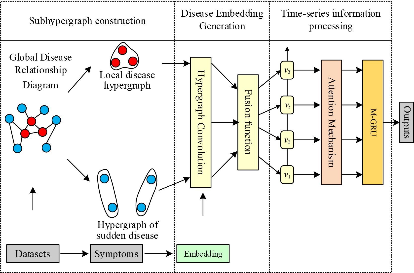
DHG4DP overall framework
SYMBOL DESCRIPTION: During a medical visit, a patient may be diagnosed with one or more conditions, which are usually indicated by specific medical codes.
Given an electronic medical record dataset {
Problem Statement: Predict the diseases that will be diagnosed in a patient’s
Since the patient possesses multiple visits, and each visit the patient is not diagnosed with exactly the same disease, a dynamic hypergraph can be obtained for the patient’s historical visits. In this section, let G = {G1,G2,⋯,G
In practice, a disease diagnosed at a single visit may be either a persistent disease or a sudden-onset disease. In order to model the fine-grained higher-order relationship between persistent and emergent diseases, for the set D
Persistent Disease:
Sudden illness:
After categorizing the diseases diagnosed at the
Localized Disease Hypergraph
Sudden illness hypergraph
In real healthcare scenarios, a disease diagnosed in a single visit by a patient may be long-standing or sudden in onset. To capture these effects, in the dynamic hypergraph learning module, this section extracts the local context as well as the abrupt context.
Local context: for each diagnostic node (i.e., the node corresponding to the diagnosed disease in the hypergraph), this section aggregates the representations of the diagnostic nodes connected to it in the hypergraph
Sudden context: for each sudden disease node, this section aggregates the representations of the diagnostic nodes connected to it in the hypergraph
The above operation captures the fine-grained higher-order relationships of diseases in the same visit, and it is obvious that there are some relationships between diseases in different visits, in order to further capture the relationships between diseases in different visits, this section designs a transfer function to extract the transfer context from the historical visits, as follows.
For sudden-onset disorders
In the case of persistent disorders, since they have been diagnosed several times in previous visits, this section provides that the representation of such disorders remains the same from visit to visit.
Using M-GRU to capture the interaction between the persistent disease representation
After that, this section uses the maximum pooling operation on the transfer output to generate the visit representation
Finally, this section utilizes the attention mechanism to calculate the impact of each visit in a patient’s history on the predicted outcome to obtain the final visit representation, as shown in the following equation:
After constructing two dynamic sub-hypergraphs in the previous subsection, this paper uses the hypergraph convolution module to process them. Before that, the inputs of hypergraph convolution are clarified.
The different relationships between disease and patient will directly lead to different impacts on the patient. Therefore, we create different disease embedding for the same disease from two aspects, respectively:
Direct disease. The disease is diagnosed directly by the patient and this embedding is recorded as Indirect disease. The disease is a neighbor of the disease directly suffered by the patient; this embedding is denoted as
For the convenience of subsequent calculations, both diseaseembedding have the same dimensions, i.e.,
After the calculation of the above two formulas, we get the two disease embedding at the time of hospitalization record
In this paper, diseases are divided into three categories in terms of temporal relationships:
Long-term diseases. The vector is denoted as Emerging associated diseases. Vector denoted Emerging unrelated diseases. Vector denoted
The attention mechanism is then used to learn the impact of the latter two disease categories on the patient’s disease embedding generation. Noting the embedding matrix as the set of embedding for diseases that neither appear in the existing disease records nor in the direct neighbors of the diseases in the existing disease records, the attention mechanism is computed as follows:
For long-term illness
Here,
After the above computation, the location-based attention mechanism is used to fuse all the hospitalization records embedding to get the final embedding
Here
The disease predictions of the model are then obtained through a multilayer perceptron (MLP) layer.
The MIMIC-III dataset was chosen for this experiment to verify the model effect, and its detailed information can be found in Table 1. This dataset has 1863 diagnostic items.
MIMIC-III data set information
| Statistical Items | Quantity |
| Diagnoses | 1863 |
| Treatment procedures | 1365 |
| Patients | 5596 |
| Dictionary size of text data | 64352 |
| Average of diagnoses | 12.8 |
| Average of treatment procedures | 4.33 |
| Average word of per visit | 2234 |
Because the purpose of this experiment is to predict the disease for which a patient will visit the clinic next, patients who have visited the clinic at least twice in the EHR data are selected, i.e., patients who have visited the clinic less than twice are deleted, and patients who have visited the clinic with both textual information and information about the diagnosis and treatment process are also selected from it.In the MIMIC-III database, four tables, DIAGNOSES_ICD, PROCEDURES_ICD, ADMISSIONS, and NOTEEVENTS, were selected from which textual information such as patient’s diagnostic code, therapeutic procedure code, information about the time of the visit, and medical advice were obtained, respectively. For the information in this paper, keyword extraction was performed using the TF-IDF method.
During the experiment, the MIMIC-III dataset is divided into training, validation, and test sets in the ratio of 6:2:2. The experimental environment settings and the selected evaluation metrics are Accuracy, Recall, and Mean F1 value, respectively. Among them, Recall represents the probability of being predicted as a positive sample among the actual positive samples, which measures the check-perfect rate, and Precision represents the degree of accuracy of prediction among the results of positive samples, which measures the check-accuracy rate. The average F1 value provides a comprehensive evaluation of the model’s prediction accuracy.
In order to verify the experimental effectiveness of the DHG4DP model, five baseline models are selected for comparison, namely, LIGHTED, INPLIM, Tr-LSTM, tBNA-PR, and TURTAM. The experimental results on the MIMIC-III dataset are shown in Fig. 2. Compared with the baseline model, the proposed model performs optimally in terms of Precision, Recall and F1 values and achieves the best prediction performance. The Precision, Recall, and F1 values have been improved by 3.8%, 2.6%, and 3.7%, respectively, when compared to the baseline model TURTAM, which performed better.
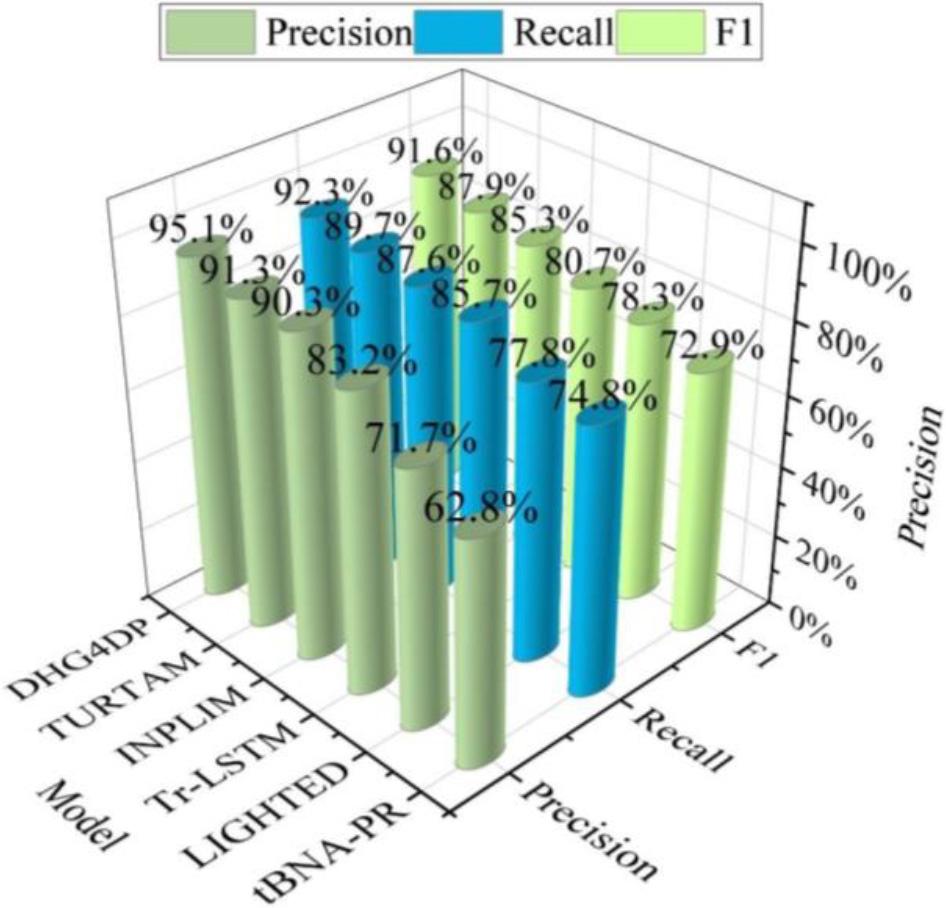
Experimental results of the MIMIC-III data set
A tertiary hospital in city A was selected for the study to reform the health management strategy. The 180 medical workers who managed health care through conventional management methods from January 2022 to November 2022 were considered as the control group. The 180 medical workers who applied healthcare management after the disease prediction network model from December 2022 to October 2023 were taken as the observation group. The statistics of the survey data are shown in Table 2.Comparing the gender data of the two groups, the difference was not statistically significant (c2=0.0311, P=0.7896). The mean age of the control and observation groups was 33.53 and 32.51 years, respectively. The difference between the age data of the two groups was not significant (t=0.8724, P=0.4116). The 1050 patients admitted during the treatment period of the control group and the observation group, respectively, were investigated as the patient group, and the difference between the gender data of the two groups was not statistically significant (c2=0.2468, P=0.6236). The control group and observation group had an average age of 53.41 years and 51.33 years, respectively. The difference between the age data of the two groups was not significant (t=0.7365, P=0.4635). In conclusion, the experimental subjects selected in this paper are suitable for control analysis.
Survey data
| Data | Group | N | M | SD | t/c2 | P | |
| Gender | Female | Observation group | 71 | - | - | 0.0311 | 0.7896 |
| Male | 109 | - | - | ||||
| Female | Control group | 69 | - | - | |||
| Male | 111 | - | - | ||||
| Age | Observation group | 180 | 32.51 | 8.22 | 0.8724 | 0.4116 | |
| Control group | 180 | 33.53 | 8.01 | ||||
| Patient gender | Female | Observation group | 506 | - | - | 0.2468 | 0.6236 |
| Male | 544 | - | - | ||||
| Female | Control group | 495 | - | - | |||
| Male | 555 | - | - | ||||
| Patient age | Observation group | 1050 | 51.33 | 12.63 | 0.7365 | 0.4635 | |
| Control group | 1050 | 53.41 | 13.11 | ||||
Before and after the reform of the health management strategy, the hospital’s health management scores, medical staff’s health knowledge scores, and the incidence of health emergencies were used as observation indicators. Among them, the health management work score was mainly determined by the hospital’s health management work score sheet, including the score of infectious disease management organization, the score of health management system implementation, the score of infectious disease reporting, the score of medical staff’s vaccination card checking, the score of hospital health care room management, etc. The score was scored using the Likert 1-10 scale method, and the score value was positively correlated with the effect of the health management work.The health knowledge score of medical staff was determined by the hospital’s questionnaire, which included knowledge of infectious diseases, methods of preventing infectious diseases, and health knowledge, etc. The total score of each item was 100, and the score was positively correlated with the health knowledge level of medical staff.Health emergencies include influenza, chicken pox, mumps, bacillary dysentery, and tuberculosis.
The final data of this study were processed using spss26.0 software before and after the reform of the health management strategy. The measurement data for hospital health management work scores and health knowledge scores of medical staff are expressed as standard deviation and tested by t.The rate of health emergencies is determined by the counting data expressed as a percentage and tested by C2. When p is less than 0.05, it means that the difference is statistically significant.
A comparison of hospital health management scores before and after carrying out healthcare management strategy reform is shown in Table 3. In the observation group, the scores of hospital infectious disease management organization (A1), health management system implementation (A2), infectious disease reporting (A3), medical staff vaccination card checking (A4), and hospital health care room management (A5) were significantly higher than those of the control group, and the differences were statistically significant (P<0.05).
Hospital health management performance ratings
| Group | N | A1 | A2 | A3 | A4 | A5 | |||||
| M | SD | M | SD | M | SD | M | SD | M | SD | ||
| Control group | 180 | 6.23 | 1.24 | 6.54 | 0.98 | 6.85 | 0.78 | 6.89 | 1.11 | 6.74 | 1.07 |
| Observation group | 180 | 9.47 | 0.33 | 9.51 | 0.16 | 9.44 | 0.24 | 9.66 | 0.32 | 9.55 | 0.29 |
| t | - | 4.485 | 2.364 | 4.514 | 4.189 | 3.367 | |||||
| P | - | 0.003 | 0.004 | 0.001 | 0.003 | 0.000 | |||||
A comparison of health knowledge scores of healthcare workers before and after carrying out healthcare management strategy reform is shown in Table 4. In the observation group, healthcare workers’ knowledge related to infectious diseases (B1), methods of preventing infectious diseases (B2), and scores of health knowledge mastery (B3) were significantly higher than those of the control group, and the difference was statistically significant (P<0.05).
Comparison of health knowledge scores of medical staff
| Group | N | B1 | B2 | B3 | |||
| M | SD | M | SD | M | SD | ||
| Control group | 180 | 55.36 | 5.36 | 61.33 | 5.85 | 59.63 | 5.77 |
| Observation group | 180 | 86.35 | 8.32 | 88.64 | 8.01 | 86.47 | 8.36 |
| t | - | 10.635 | 11.587 | 9.658 | |||
| P | - | 0.000 | 0.000 | 0.000 | |||
A comparison of the incidence of health emergencies before and after carrying out the reform of healthcare management strategies is shown in Table 5. The incidence rate of health emergencies such as influenza (C1), chickenpox (C2), mumps (C3), bacillary dysentery (C4), and tuberculosis (C5) among the patients in the observation group was 1.9%, which was significantly lower than that of the control group (4.95%), and the difference was statistically significant (P=0.016<0.05).
The incidence of emergency health events was compared
| Group | N | C1 | C2 | C3 | C4 | A5 | Total incidence |
| Control group | 1050 | 25 | 9 | 10 | 4 | 4 | 52(4.95%) |
| Observation group | 1050 | 9 | 7 | 4 | 0 | 0 | 20(1.9%) |
| c2 | - | - | - | - | - | - | 6.358 |
| P | - | - | - | - | - | - | 0.016 |
In this paper, we combine graph theoretical methods and utilize graph neural networks for in-depth analysis of medical and health records as a way to facilitate the management of healthcare. The study’s dynamic hypergraph network-based disease prediction model outperforms the five baseline models in prediction performance. Compared to the best-performing baseline model, the precision, recall, and F1 values of this paper’s model have been improved by 3.8%, 2.6%, and 3.7%, respectively. Applying this paper’s constructed disease prediction model to medical work significantly improves the hospital health management work score, health care workers’ health knowledge score, and the incidence of health emergencies compared to the traditional health management model, with a P value less than 0.05. It shows that the disease prediction model applied to medical work helps to improve the effectiveness of health management.
Source: 2023 Henan Provincial Department of Science and Technology Soft Science Project;
Project Title: “Evaluation Study on Home-Based Bedside Care Services in Henan Province”;
Project Number: 242400410363.