Deep Learning Algorithms for Efficient Recognition in Biometric Image Classification

Online veröffentlicht: 17. März 2025
Eingereicht: 27. Okt. 2024
Akzeptiert: 09. Feb. 2025
DOI: https://doi.org/10.2478/amns-2025-0163
Schlüsselwörter
© 2025 Jing Ning, published by Sciendo
This work is licensed under the Creative Commons Attribution 4.0 International License.
In recent years, image recognition algorithms based on deep learning have been widely used in many fields, including biometrics. Biometrics refers to the technology of authentication or identification by analyzing the physiological or behavioral characteristics of biological individuals, such as fingerprint recognition, face recognition and iris recognition [1-3]. The development and application of these technologies are crucial for the protection and security of important information, and the application of image recognition algorithms based on deep learning in biometrics has become an area of great interest [4-5]. Traditional biometric identification and classification methods are mainly based on traditional machine learning methods, such as support vector machines and random forests. However, these methods often suffer from insufficient accuracy and robustness when dealing with complex biometric data [6-9]. In order to solve these problems, deep learning techniques have been gradually introduced into biometric identification and classification algorithms in recent years, and significant research results have been achieved.
Deep learning is a kind of machine learning, the core of which lies in automatically learning the representations and features of data through algorithms and transforming data into meaningful information. The use of deep learning algorithms allows computer systems to extract different levels of feature representations from input data to achieve more accurate recognition [10-13]. In biometrics, the basic principle of deep learning is to construct a deep convolutional neural network to analyze biometric images at the pixel level, learn how the human brain processes and recognizes biometric features, and ultimately transform the image into a “fingerprint” that can be described and compared [17-17].
Finizola, J. S. et al. provide a detailed description of biometrics, including its features, applications, impact and shortcomings, and examine the differences between traditional machine learning models and deep learning paradigms, in particular convolutional neural networks and autoencoders for facial recognition [18]. Abinaya, R. et al. implement user identification in view of facial features. The local binary pattern and grayscale covariance matrix image features were extracted by various deep learning classification techniques such as convolutional neural networks and effectively represent the facial and skin regions of the user and classify their facial images. The experimental results proved the excellent accuracy of Convolutional Neural Networks [19]. Mehraj, H. et al. analyzed the biometrics research using deep learning to derive its advantages and potentials and provided a comprehensive overview of migration learning for deep biometrics. Their study addressed all the strategies and datasets used and their accuracy and discussed the challenges encountered in applying biometric models and their direction of development [20]. Zulfiqar, M. et al. presented a face recognition system with convolutional neural networks, which achieves face recognition by detecting it using Viola Jones face detector, and experimental results specified that deep face recognition in the biometric automatic authentication system showed great effectiveness [21]. Ortiz, N. et al. emphasized that biometrics are often used to provide authentication information in security systems. However, there are individual features that are difficult to access by means of attributes. Therefore, some machine learning methods for biometric pattern recognition were elaborated [22]. Singhal, N. et al. unfolded a review of the comparative study of face recognition techniques and their hybrid combinations, not only analyzing the datasets in the field and the prospects and challenges in this field but also emphasizing deep learning-based facial recognition algorithms [23]. Selitskaya, N. et al. reveal that there are problems in machine learning in the field of face recognition due to illuminations, emotions, etc., which affects the accuracy of the recognition, as well as the deep neural network for such effective solutions [24]. Medjahed, C. et al. proposed and trained a multimodal biometric system using convolutional neural networks and K-nearest neighbors aimed at individual recognition. Performance experiments in extreme cases were carried out, and the results showed that the proposed system outperforms all the current mainstream biometric verification techniques [25]. Minaee, S. et al. investigated the deployment of a deep learning model for biometric identification and also demonstrated the advantages and potentials that this model embodies in various applications. It also discussed the challenges faced by deep learning models for biometric identification and its future research directions [26].
In this paper, we first introduce the layers frequently used in convolutional neural networks turn, which consist of multiple convolutional layers, pooling layers and fully connected layers, with a nonlinear mapping layer and a normalisation layer added after the sampling layer to prevent overfitting. Next, the DenseNet-121 model used in this paper is introduced, which belongs to the DenseNet family and covers four dense blocks and three transition layers. The feature extraction work on biological images is performed using DenseNet-121, and then chaotic initialisation is introduced, which is used to optimise the initial population in the FDA, enabling the FDA to find the global optimal solution faster and speeding up the convergence of this algorithm. Finally, the FDA algorithm optimised by multiple population mechanisms is proposed, and the parameters optimised in the FDA are applied to the ELM using the method of search agent mapping, which is put into the biometric features to classify the biometric features. The excellent performance of the convolutional neural network model and the optimized ELM classifier has been verified experimentally.
A convolutional neural network consists of multiple convolutional layers, pooling layers, and finally, a fully connected layer.In order to prevent overfitting and speed up loss convergence, a nonlinear mapping layer and a normalization layer are usually added after the sampling layer.Next, the layers that are commonly used in convolutional neural networks are introduced in turn.
Usually, convolution is a mathematical operation of two real functions with the expression:
In CNN [27], the first parameter
In deep learning, the inputs to a convolution are usually high-dimensional arrays, and the resulting convolution kernel produced by the operation is also a high-dimensional array. For example, taking a two-dimensional image
Since the convolution operation is commutative, its equivalent:
Through convolutional operations, the original information will be increased, and the noise will be reduced. In the convolutional layer of CNN, a convolutional kernel extracts only one kind of biometric map of the input information. In order to be able to extract enough biometric maps, multiple convolutional kernels are needed in each layer. These parameters related to the convolutional kernel are the training parameters, which will be continuously updated throughout the training process of the network.
The pooling layer, also known as downsampling, makes use of the principle of local correlation of images to subsample the biometric images, with the aim of reducing the feature dimensions and reducing parameters while retaining the useful information so that the final feature representation maintains some invariance (selection, translation, scaling, etc.). In CNN, common pooling algorithms are maximum pooling, average pooling, and random pooling. Maximum pooling means taking the maximum value for all feature points in the domain, average pooling is averaging the feature points in the domain, and random pooling is between average pooling and maximum pooling, which only randomly selects the elements in the feature map according to the size of their probability values. According to the relevant theory, average pooling reduces the valuation error caused by the restricted domain size during feature extraction, while maximum pooling reduces the estimated mean shift caused by the parameter error of the convolutional layer. Regardless of which pooling function is used, it serves to keep the output as constant as possible when the input makes a small translation. For example, for the invariance of translation, when we translate the input by a small amount, the output value does not change after passing the pooling function.Local translation invariance is a significant attribute, particularly when we are interested in whether a feature appears or not but not exactly where it does.
The Relu layer is a layer that has unsaturated nonlinear mapping [28] that extracts the biometric feature from the convolutional layer and produces the unsaturated nonlinear mapping value that corresponds to that biometric feature. In previous convolutional neural networks, saturated linear functions such as sigmod, tanh, etc., are usually used for nonlinear transformation, but such nonlinear functions contain many redundant parameters. When using gradient descent to optimize the loss function, we choose the unsaturated nonlinear function Relu in order to obtain faster convergence and prevent the gradient from vanishing. For a sample set of labelled data (
The purpose of the normalization layer is to enhance the contrast of the biometric map, similar to increasing the contrast of an image. The current algorithm often used in the normalisation layer is Local Response Normalisation (LRN), which mainly achieves local competition between neighbouring biometric features in the same biometric map, as well as biometric features in the same spatial location of different biometric maps, by subtraction and division normalisation of the local biometric map, which makes the background and the main content of the image distinctly different.
The ResNet model is a deep convolutional neural network [29], which effectively solves the gradient vanishing and model degradation problems in deep network training by introducing a residual learning framework. Traditional deep neural networks suffer from the problem of gradient vanishing, i.e., the gradient will gradually decrease and eventually vanish during the backpropagation process, leading to difficulties in the training of deep networks. The core innovation of the ResNet network structure is the use of residual connectivity, which allows the network to pass inputs to the subsequent layers, thus simplifying the learning process and making it possible to construct extremely deep network models. However, ResNet still has some drawbacks. Its relatively complex connection structure can lead to a high number of network parameters, which increases the complexity and computational cost of the model. In addition, while jump connections help in gradient propagation, in some cases, these connections may still lead to problems where gradients vanish or explode.
In contrast to ResNet’s residual blocks, the DenseNet model uses a dense connectivity mechanism that connects a piece of input directly to the output. In DenseNet, each layer is directly connected to all previous layers, allowing features to flow freely through the network. This dense connection strategy effectively mitigates the problems of gradient vanishing and information loss in deep learning models by optimising the flow and reuse of features, and improves the efficiency of the model’s parameter usage and its generalisation performance to new data. Specifically, DenseNet adopts a modular structure called “dense block”. Within a dense block, each layer is directly connected to previous layers. This fully-connected approach facilitates the wide dissemination of features and improves feature utilisation and information flow in the network. In such a dense block, layers are tightly connected by superposition, forming a highly integrated feature processing network. Let the dense block have L layers. The input feature map of the first layer is noted, and then the output feature map of the Xth layer can be expressed as:
Where
The DenseNet-121 model used in this paper belongs to one of the DenseNet families. It covers four dense blocks and three transition layers. The network model is depicted in Fig. 1. In these dense blocks, each layer achieves direct connections with the previous layers, allowing each layer to directly access and utilize the feature maps of the previous layers.This design is effective in promoting the efficient circulation and reuse of feature information, as well as reducing the total number of parameters in the model, improving the efficiency of parameter usage.

Example of network structure
In this study, feature extraction work on biological images using DenseNet-121, proposed FDA algorithm optimised by chaotic strategy, multiple swarm mechanism, whereas the optimised parameters of FDA are later applied to ELM using search agent mapping method, input features, and classification.
Therefore, this study introduces chaotic initialization to optimize the initial population in FDA, accelerating the convergence of the algorithm and finding the global optimal solution faster.In order to maximize the optimization performance of chaotic initialization for the initial population in FDA, in this study, the chaotic function in the Logistic map algorithm is used.
STEP 1: Add Chaos Theory and invoke Logic Mapping to expand the search for dry stream populations to form a new sequence of populations:
STEP 2: In order to further optimise the FDA’s optimisation seeking capability especially for the selection of ELM models, this study introduces multiple population mechanisms for the FDA. The initial population will be replicated into
The tributary NEIGHBOR of the flow algorithm has a better balance of its exploration and exploitation capabilities with offset Δ. As the iteration deepens, Δ changes from large to small, shifting from extensive exploration to exploitation of optimal values. However, when a more optimal tributary does not exist in a certain iteration, the stem flow shifts to some other stem or flows to the current optimal stem, as in Eq. (8). In this process, the algorithm is not able to balance the ability of exploration and exploitation, which can easily lead to individual deviation from the optimal solution or fall into the local optimum, for this reason, we introduce fuzzy logic.
Firstly, the normalised fitness value of the current stem flow is calculated:
where
The fuzzy logic uses the generation of Δ
This study uses the technique of search agents to directly optimize the ELM for the number of input nodes N and the number of hidden layer nodes M. Being two key parameters that determine the structure of the network. They are not capable of undergoing modification during the operation of the network. Common algorithms that use ELM set N and M manually and choose the best configuration after repeated experiments. The search agent mapping approach pre-sets the maximum structure of the network, inputs both the N number of input nodes and the M number of hidden layer nodes as independent parameters into the optimisation algorithm for optimisation, and performs a dichotomous operation on the final result, mapping the result to either 0 or 1 to determine whether the current node is active or not. The combination of multiple swarm strategies, diverse populations provided by the chaotic initialisation strategy and the repeated iteration process serve to screen out invalid input features and optimise the number of hidden layer nodes, avoiding network bloat and eliminating the tedious process of manual setup.
Considering each input node and hidden layer node as independent parameters, M and N are pre-maximised and jointly put into the optimisation algorithm for iterative optimization.The values of the weight and bias parameters are kept constant as weights between the input and hidden layers of the ELM, and the bias of the hidden layer. Parameters representing the input and hidden layer nodes are binarily differentiated after the optimisation is complete to determine whether to activate the specified nodes. In this study, we constrained the search range of each particle to be in [-1, 1], and the Ceil function was used to map the two optimised node parameters to 0 and 1. When the node parameter pancreatic maps to 1, it means that the node is activated, and vice versa, it represents freezing the node. Subsequently, the weights and biases are rearranged according to all the activated node parameters, which can always ensure that there is no dimensional mismatch during the ELM training process, and at the same time, an alternative way to optimise the number of input nodes and the number of hidden layer nodes is achieved.
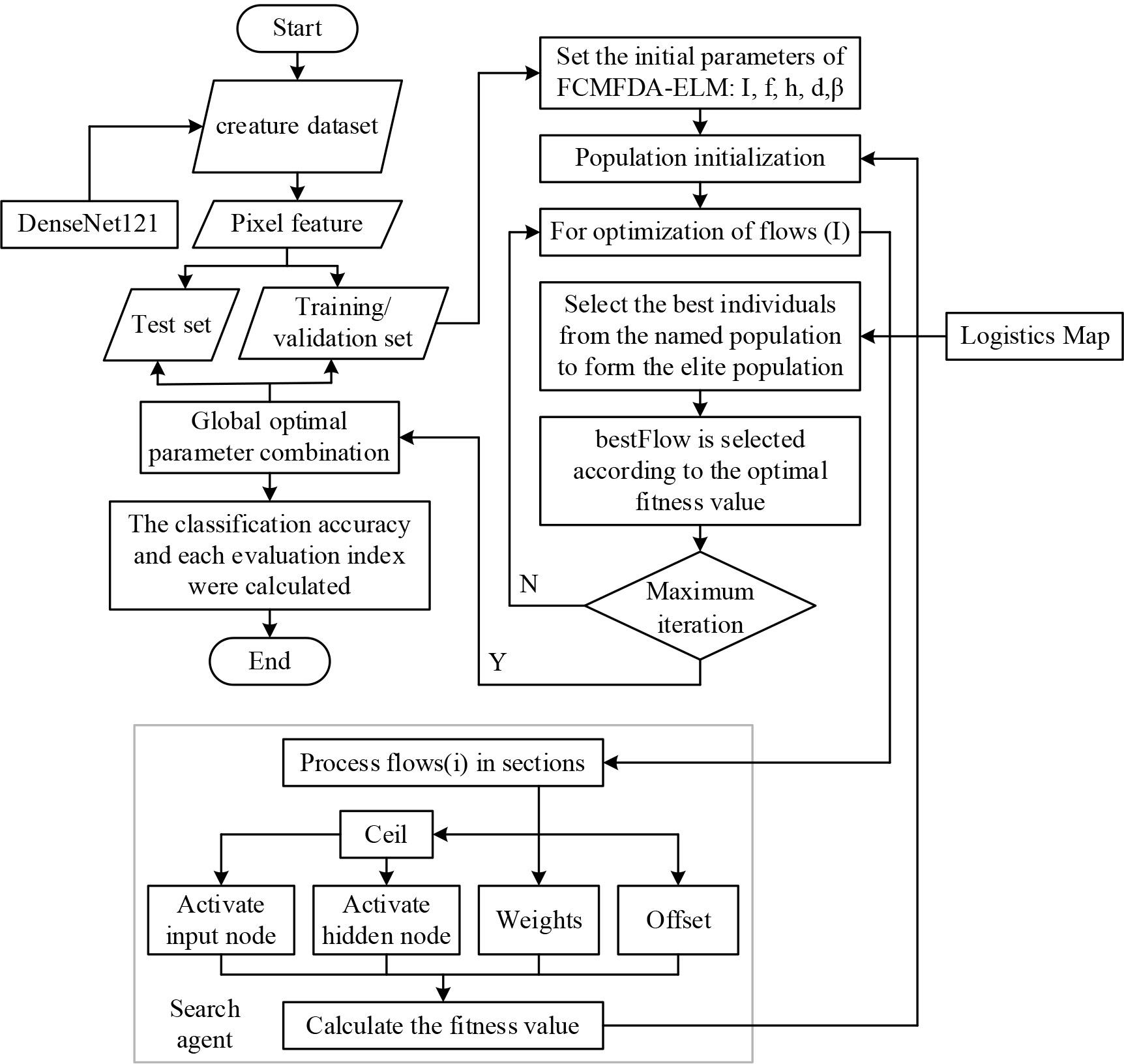
The main factors affecting the prediction performance of ELM are input features, weights between the input layer and the hidden layer, bias of the hidden layer, number of nodes in the hidden layer, and weights between the hidden layer and the output layer. Among them, the weight between the hidden layer and the output layer is obtained directly from the network training. In this study, chaotic initialisation and multiple swarming mechanisms are used to obtain a more random and more generalised initial population, and the better initial population determines the weights between the input layer and the hidden layer and the bias of the hidden layer. Introducing fuzzy logic, the FDA balances exploration and exploitation capabilities, avoiding individuals from falling into local optima. At the same time, the search agent mechanism is added to the optimisation of the FDA algorithm, which synchronously optimises the number of input nodes and the number of hidden layer nodes of the network, completes the selection and screening of important biometric features, and the setting of hidden layer nodes, which improves the accuracy and stability of the biometric image classification algorithm. The classification accuracy of the validation set is used as the adaptation value of the algorithm. Repeatedly iterating, as the fitness value continues to approach the target optimal value thus selecting the best combination of parameters. The final flow diagram of the biometric image classification algorithm using convolutional neural networks and FCMFDA-ELM is shown in Fig. 2, and the overall operation flow of the algorithm is as follows:
Use ImageNet Migration Learning DenseNet-121 network to extract features from the biological images in the dataset and perform appropriate dimensionality reduction operations to take the category of the biological image as the label. Divide the extracted dataset features into an 8:1:1 training set, validation set, and test set, where the training set is used to train the ELM network, the validation set is used to calculate the fitness value to feed back the optimisation status of the network, and the test set returns the final metrics for evaluating the algorithm performance. Set the initial parameters of the algorithm: the initial number of populations M for multiple swarm strategies, the number of search agents for each population, the maximum number of iterations I, the maximum number of features F, the maximum number of hidden layer nodes H. Finally, the search agent dimension is jointly represented by the above multiple parameters as D-F+H+(F*H)+H, as well as the number of tributaries β in the FDA algorithm. According to the search agent, the number of input nodes and the number of hidden layer nodes will be accompanied by the weights and bias parameters together into the FCMFDA in accordance with the fuzzy logic optimised FDA process to start the optimisation search. The Apply the parameters of step 5 on top of the ELM, solving for the fitness value on the validation set for all Detect whether the current iteration has reached the maximum number of iterations. If the maximum number of iterations has not yet been reached, it will return to step According to the algorithm finally obtained 6 Parameters in the ELM are resolved and applied to the test set to calculate various algorithm evaluation indexes to assess the performance of the algorithms of this study. He convolution network and optimized elm classification algorithm
The experiments specifically used ResNet50, ResNeXt50, Efficient Net, and DenseNet121 models in the dataset for training and evaluation.
Dataset: 20 egg samples randomly selected for both eggshell colour and main biometric features, one egg for one biometric category. Each category contains 100 eggshell images, different CNN models are used for individual recognition of biometric features of eggs and the results are evaluated.
The recognition accuracies of the four CNN models during 200 epochs of training are shown in Figure 3. Among them, the accuracies of Efficient Net and DenseNet121 models are kept at a high level overall. This means that they process the data better on this dataset. The Loss curves of the four CNN models during 200 epoch training are shown in Fig. 4, and the Loss value of the DenseNet121 model is much lower than the other three models. Among them, DenseNet121 is slightly better than Efficient Net, whose accuracy eventually converges to 97.26% with a Loss of 0.66.
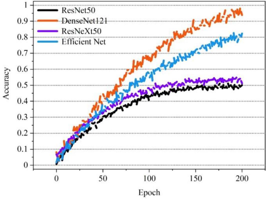
Model accuracy curve
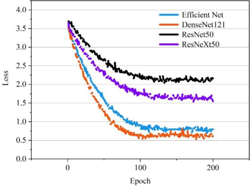
Model loss curve
The models are tested on the test set, and their accuracy, precision, recall, F1-score, and Kappa results are shown in Figure 5. It can be seen that the DenseNet121 model scores higher than the remaining three CNN models in all metrics, which indicates that it has the best performance in the task of biometric recognition of eggshell images. However, DenseNet121 only obtained 88.85% accuracy on the test set, and the remaining precision, recall, F1-score, and Kappa scores were 83.17%, 87.15%, 81.13%, and 82.61% respectively.This is a significant difference from the results of the training set, which indicates that the model has some overfitting and poor generalization problems. The insufficient data sample size may cause it. For the training on the dataset of 20 egg categories, the model is not yet able to show the best generalization performance. Later on, we can consider using a larger dataset for training, as well as adjusting the training strategy of the model.
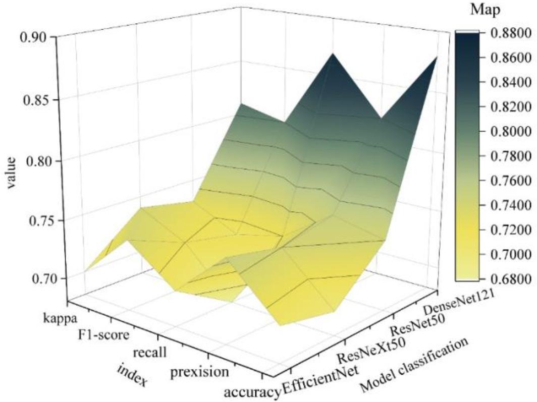
Various evaluation results of different models
The ROC curves of each model were further plotted, and the results are shown in Figure 6. It can be seen that among the four models tested, the curve of the DenseNet121 model is closest to the upper left corner, implying that the AUC value is the largest and its classifier has the best performance. The results also indicate that the DenseNet121 model is more effective in extracting eggshell organism features than the remaining 3 CNN models.
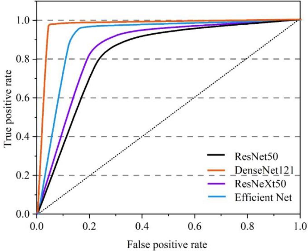
Roc curve of different models
The performance of the models is also reflected in the amount of computation (MACs), the number of parameters and the speed, and the results of the comparison of the computational performance of each model are given in Table 1. The MACs of the DenseNet121 model are 0.42 G, the number of parameters is 21.02 M, and the speed of computation is 28.14 ms. It is noteworthy that the Efficient Net model has the smallest number of parameters (2.56 M), which can reflect certain advantages in the application of pursuing model lightweighting. The computational performance of Efficient Net, ResNet50, and ResNeXt50 models are close to each other, and they are used as alternative models for the backbone network of biometric feature extraction, but the priority in the process of biometric feature extraction is to ensure the recognition accuracy before considering the computational performance of the models. Therefore, the behavior of DenseNet121 as a backbone network for extracting biometric features is correct in this paper.
| Model name | MACs(G) | Parameter quantity(M) | Speed(ms) |
|---|---|---|---|
| ResNet50 | 0.27 | 24.56 | 39.56 |
| ResNeXt50 | 0.31 | 23.98 | 34.51 |
| Efficient Net | 0.15 | 2.56 | 31.28 |
| DenseNet121 | 0.42 | 21.02 | 28.14 |
Images of 450 biometric samples of pests (50 per class) were collected in the laboratory. Class 1 to 9 are rice leaf borer, bean field moth, golden tortoise, mole cricket, cotton bollworm, beet noctuid moth, small groundhog, sooty bollworm, and stickleback, in that order. The 450 test samples were classified and identified using the CNN-based and optimised ELM classifier, and finally, the results of the confusion matrix of this classifier on the test set were plotted, and the results are shown in Fig. 7, where each column represents a category label, and the sum of the numbers in each column represents the number of biometric images of the pests in that category. The 50 images of categories 1 and 5 in the test set have a classification accuracy of 100%, while category 3 has the lowest classification accuracy of 80%. Due to the small differences in the pest images, the overall classification accuracy of the model nevertheless reached 92.22%. This indicates that the optimized ELM classifier has good classification performance, and the CNN-based and optimized ELM classifiers can be directly used for biometric image classification and recognition tasks.
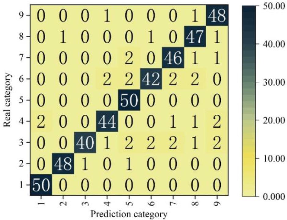
The confusion matrix of the densenet121 model
In this section, the classification effectiveness of the optimised ELM classifier is verified by using sequentially increasing 100, 200, 300, 400,500, 600, 700, 800,900,1000,1100 pest image samples respectively.The experimental results of the optimized ELM classifier are shown in Fig. 8. From the experimental results given in Fig. 8, and it can be seen that the optimised ELM classifier proposed in this paper has no significant change in the correct classification rate with the increased database, which proves the stability of the classification algorithm proposed in this paper.
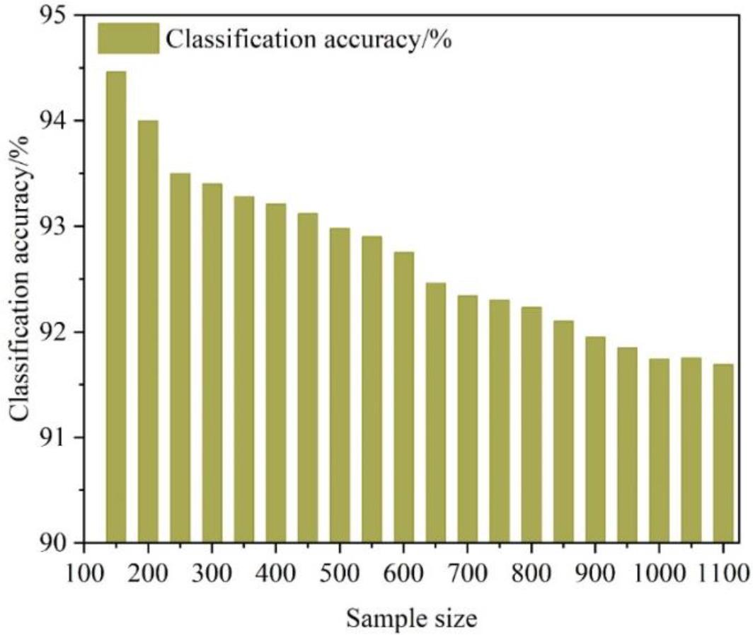
Classification accuracy
The article introduces the biometric recognition method and optimises the biometric image classifier.
The accuracy of the DenseNet121 model in recognizing the biometric features in the image is maintained at a high level, much higher than the remaining three models, and the loss value is much lower than that of the other three models, with its accuracy converging to 97.26% and loss converging to 0.66 when the Epoch is 200, and the ROC curves of the DenseNet121 model present the results of the best performance of the classifier. The AUC value is the highest, and the classifier performance is the best. It reflects the high efficiency of the DenseNet121 model for biometric feature extraction.
In the image recognition classification experiment of biometric samples of pests, the classification accuracy of categories 1 and 5 in the test set reached 100%, and the overall classification accuracy of the model reached 92.22%. When the number of samples increases sequentially, the classification effect of the optimised ELM classifier does not change significantly, proving the stability of the proposed classification algorithm in this paper.It shows that the optimized ELM classifier has good classification performance and verifies the practicality of the CNN-based and optimized ELM classifier, which can be directly used for biometric image classification and recognition.
Science and Technology Plan Project of Liaoning Province: Research on the Application of Device Health Management System based on Deep Learning (Project number: 2023JH2/101700315).
Liaoning Provincial Department of Education General Project: Research on the Fusion Technology of Multimodal Biometric Identity Authentication in Intelligent Security (Project number: JYTMS20230709).