Research and optimisation of a deep learning model for positive thinking meditation based on bio-signal processing

Online veröffentlicht: 17. März 2025
Eingereicht: 30. Okt. 2024
Akzeptiert: 05. Feb. 2025
DOI: https://doi.org/10.2478/amns-2025-0157
Schlüsselwörter
© 2025 Yukun Zhu et al., published by Sciendo
This work is licensed under the Creative Commons Attribution 4.0 International License.
Positive thinking meditation, as an ancient practice, has demonstrated many positive effects and benefits in modern scientific studies [1-2]. Through stress management, emotion regulation, cognitive function enhancement, and physical and mental health improvement, mindfulness meditation provides an effective way for people to self-regulate and improve their quality of life. However, scientific research is still in the process of deeper exploration, and more findings on positive thinking meditation will reveal to us its wider application areas and potentials [3-6].
First of all, positive thinking meditation produces a series of positive effects on human physiology. Meditation can reduce the body’s secretion of stress hormones and enhance immunity [7-8]. At the same time, meditation can also promote the activity of neurons in the brain, improve cognitive and memory functions, and increase the volume of gray matter in the cerebral cortex and temporal lobe, reducing the risk of degeneration of brain functions. Secondly, positive thinking meditation can also positively affect individuals psychologically [9-12]. Positive thinking meditation can break the “past, present and future”. The past and future often lead to speculation, judgment and uncontrollable emotional fluctuations about our situation, while positive thinking meditation allows people to return their attention to the present and the here and now and reduces anxiety and internal pain [13-16]. Positive thinking meditation can improve people’s awareness of their own emotions and thoughts, improve self-control and self-regulation in daily life, and reduce tension and anxiety by making people aware of changes in the inner details of the body [17-20].
In this paper, 100 subjects without any experience in positive thinking meditation were recruited through screening to participate in a positive thinking meditation experiment. The EEG and infrared signals of the subjects were collected by using self-designed optical polar plates and other related equipment, and then formed the biosignal dataset required for the subsequent study after noise reduction by the independent component analysis method. In order to scientifically plan the training strategy of mindfulness meditation, this paper constructs a stage classification model of mindfulness meditation by combining deep learning and short- and long-term memory neural networks and conducts simulation experiments on the subject’s biosignal dataset to validate the effectiveness of the model for the recognition of the classification of various stages of mindfulness meditation. Regarding the problem of misidentification of the stages of positive thinking meditation caused by uneven data distribution, this paper adopts the data enhancement method of cyclic displacement to increase the diversity and richness of the data so as to improve the model’s generalisation ability and recognition accuracy. Aiming at the shortcomings of deep learning models and traditional data enhancement methods, this paper constructs an integrated network model of migration learning with the MobileNetV2 model, RestNet50 network model and Xception model to further improve the classification and recognition ability of the model for each stage of positive thinking meditation. Through experiments and analyses on the subject’s biosignal dataset, the integrated network model based on transfer learning is verified to be effective in improving the classification and recognition performance of each stage of positive thinking meditation relative to other methods, such as deep learning models. It provides a useful reference for training in positive thinking meditation.
Before the beginning of the experiment, the demographic information of all the subjects was collected. The main information contained the age of the subjects, whether they had mature experience in positive thinking meditation, etc. 100 subjects without any experience in positive thinking meditation were recruited through screening, with 50 males and 50 females [21]. The psychological state of the subjects was normal, and the average age of the subjects in the experimental group was 24.6 years old. All subjects did not suffer from mental diseases and were in good health.
The brain area concerned by this positive thinking meditation experiment is mainly located in the bilateral prefrontal lobe, so the design of the light pole plate covers the area where the prefrontal lobe is located. This experiment needs to design the light pole plate by itself, and the structure of its design is shown in Fig. 1, which includes 8 light sources (red numbers 1-8, wavelengths of 720 nm and 870 nm, respectively), which are indicated by the 8 transmitting probes. 16 receiving probes (blue numbers 1-16). Maintaining a fixed distance of 5 cm between the individual probes, this setup will result in the formation of detection channels between each transmitting probe and each receiving probe, forming a total of 28 channels (green straight lines). The electrode was placed in the prefrontal region of the subject’s head, and the entire electrode was attached to the subject’s head using a black hair band.
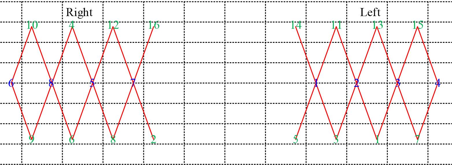
Light plate structure design
This experiment was conducted in the laboratory of the Institute of Biophysics, and it was arranged that different subjects sat in the middle of a couch during the positive meditation experiment, where the main subject #1 sat behind the couch and recorded the NIRS data, and another main subject #2 sat in front of a table to collect the EEG data [22].
Simultaneous recording of EEG and f NIRS can increase the amount of data and may be particularly useful for some brain-computer interface applications as it helps to capture changes in the activity of biological signals such as EEG and haemodynamics corresponding to a single task. Just as methods for recording brain activity continue to evolve, so must techniques for decoding multiple data streams. Figure 2 shows a sequence of oxygenated hemoglobin concentration over time for a channel during an experiment. In the lower part of Figure A-H are the eight transmitting sources, and 1-16 are the detecting receiving sources, thus constituting 28 channels. The sequence of oxyhaemoglobin concentration over time for the black and red channels is shown, where the horizontal axis represents the time (s), and the vertical axis represents the change in oxyhaemoglobin concentration for two of the channels after the change in light intensity is converted to a change in oxygen concentration by a modified Lambert-Beer law hysteresis.
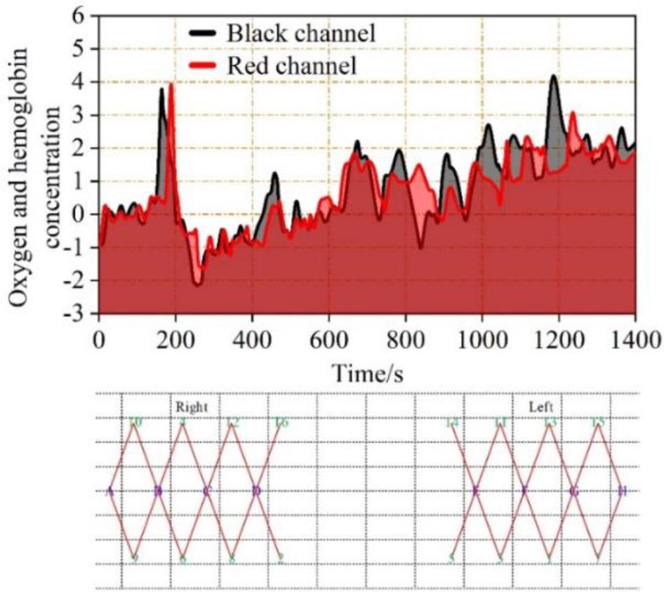
The sequence of changes in concentration of oxygen and hemoglobin
The acquired signal is first band-pass filtered from 1-100 Hz to remove motion artefacts from the signal, and then 50 Hz trap filtering is performed to remove industrial frequency interference from the power supply. Raw EEG data collected from the scalp usually consists of a mixture of useful signals and irrelevant artefacts. Theoretically, these two are considered to be independent of each other, so the artefacts can be effectively separated using an independent component analysis (ICA) method.
The time-domain waveform of the original EEG signal is shown in Fig. 3, where (a) is the signal time-domain waveform, with the horizontal axis indicating time and the vertical axis indicating the relative amplitude change of the signal. (b) is the signal frequency domain graph, it can be clearly seen from the original EEG frequency domain signal that there is an obvious 50 Hz industrial frequency interference in the signal.
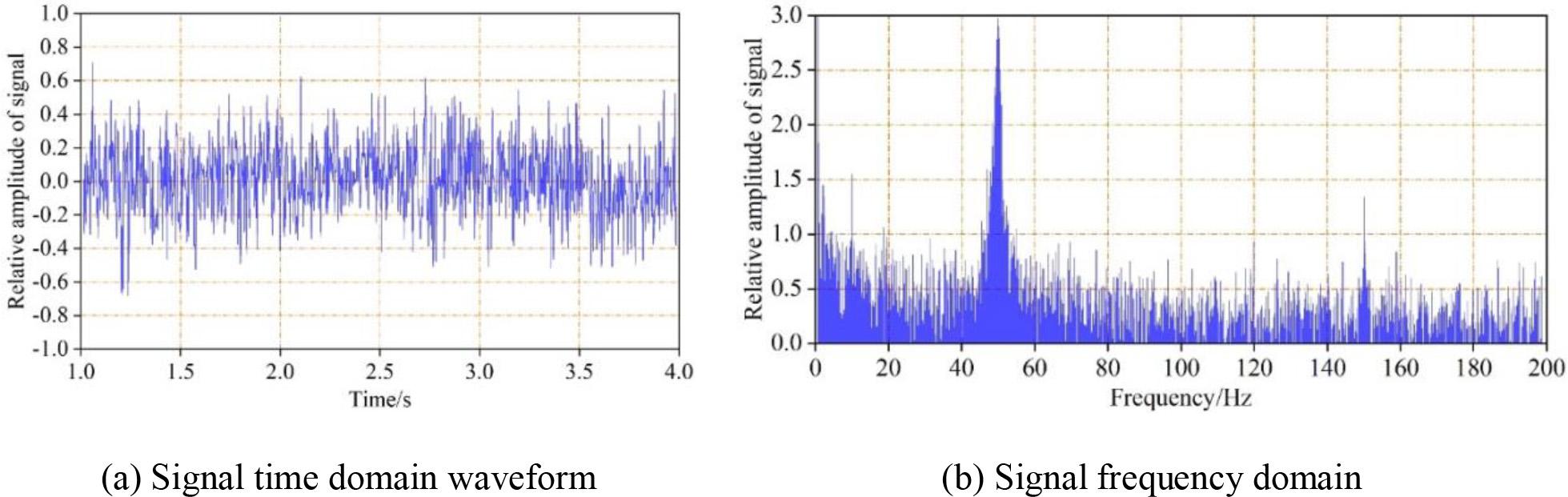
Original brain electrical signal time domain and frequency domain waveform
The processed EEG waveform is shown in Fig. 4, where (a) is the signal time-domain waveform, with the horizontal axis indicating time and the vertical axis indicating the relative amplitude change of the signal. (b) is the signal frequency domain graph, and it can be seen from the processed EEG signal graph that the 50 Hz industrial frequency interference has been significantly eliminated.
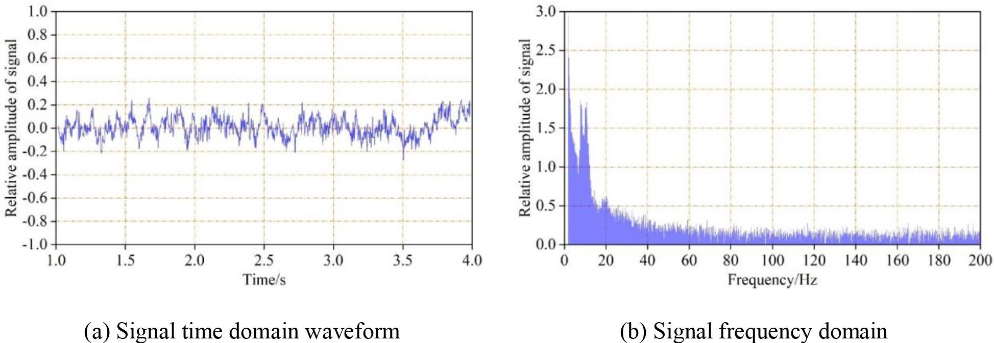
The time domain and frequency domain waveform after processing
For f NIRS data with fixed task states [23], with insufficient a priori assumptions, independent component analysis (ICA) is considered to decompose the meaningful neural activity components, while ICA methods can also strip out various types of noise components to achieve purification of f NIRS data [24]. ICA, as a data-driven method, attempts to use the ICA method to separate for noise removal. The current fNIRS-based ICA denoising method is basically temporal ICA, which is based on the temporal structure of the ICA method to make the original data under the base vector projection as free of linear correlation on time delay as possible, and the calculation formula can be written as:
The problem then boils down to coming to find a set of bases, the covariance matrix of the time delay is diagonal, and the objective function can be defined as:
The objective function
It is assumed that the temporal activity of noise and the neural temporal activity of interest for the meditation experiment are independent of each other and that the observed recorded blood oxygen signal consists of a linear summation of the changes in blood oxygen concentration due to these noise and neural activities paired with different combination coefficients:
Where
Where
Fig. 5 shows a graph of the oxygenated haemoglobin concentration of a subject over time, calculated by the Lambert-Beer law. (a), (c) and (e) are graphs of the oxygenated haemoglobin concentration of the channel monitored by H-probe No. 9, the light source of the right brain of the subject’s positive thinking meditation, respectively. (b), (d), and (f) are graphs of the changes in oxyhaemoglobin concentration in the channel monitored by the subject’s positive mindfulness meditation left brain light source C-probe No. 7. a and b are data from the subject’s first positive mindfulness meditation, c and d are data from the subject’s third positive mindfulness meditation, and e and f are data from the subject’s eighth positive mindfulness meditation. At the time of the first positive thought meditation experiment, subjects experienced a substantial change in blood oxygen concentration in the aware breathing phase, several more pronounced fluctuations in the limb awareness phase, and strong changes in blood oxygen concentration from baseline in several other major phases compared to the pre-resting phase. As the number of positive meditation training sessions increased, the blood oxygen concentration gradually leveled off. This, to some extent, justifies the identification of the phases of positive thinking meditation through the signals of blood oxygen concentration changes.
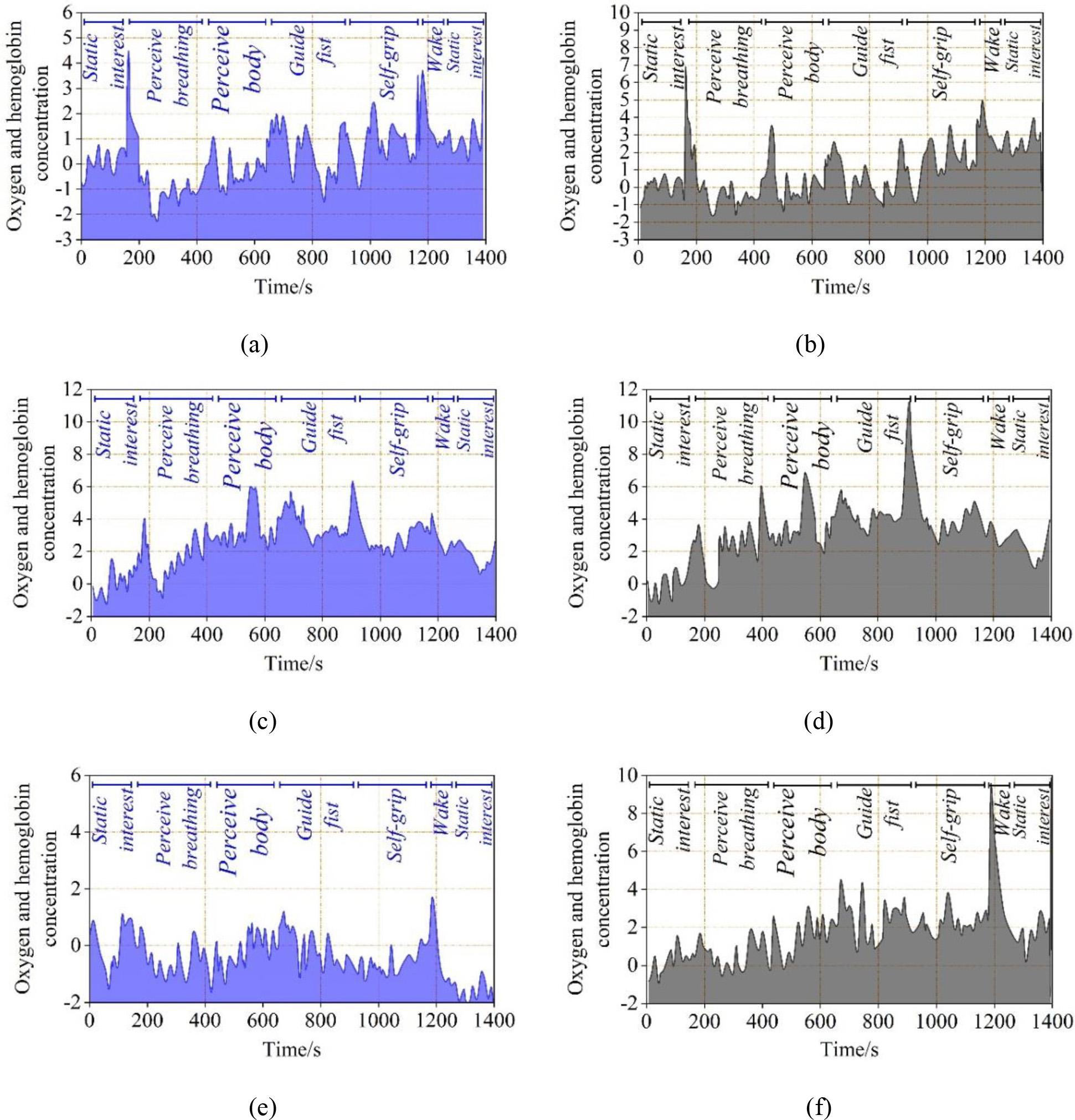
Changes in the concentration of oxygen and hemoglobin
After the processing operations described above and the processing of each meditation stage, the EEG and NIR data from the 8 meditation sessions of 100 subjects were divided according to each person per each stage to produce a dataset.
CNN is a feed-forward neural network inspired by the biological sensory field mechanism, with three structural properties: local connections, weight contributions, and convergence. CNN mainly consists of four parts: convolutional layer, pooling layer, activation function, and fully connected layer.
Convolutional layer
As the core component of CNN, the role of the convolutional layer is to extract a locally convergent feature in the input sample through convolutional operation. Specifically, each convolutional layer contains multiple convolution kernels, and the convolution operation is equivalent to moving the convolution kernels over the input samples in a particular way and summing the product between the corresponding points. At the same time, when the size of the input feature map and the size of the convolution kernel is constant, the size of the feature map obtained after convolution is affected by the movement compensation of the convolution kernel and whether or not edge filling is performed.
Assuming input feature map size
Pooling Layer
The pooling layer is another key component of CNN, which is mainly used to compress the features through feature dimensionality reduction, and at the same time, it can reduce the network complexity and the number of network parameters and prevent the model from overfitting. It should be noted that the pooling layer does not have any parameters, and the pooled features have translation invariance, scale invariance and rotation invariance. The commonly used pooling methods include average pooling and maximum pooling, which are achieved by averaging and maximising a certain region of the input feature map, respectively.
Activation function
The core role of the activation function is to enhance the nonlinear representation of the model, thus improving the model’s ability to fit the data. In CNN, commonly used activation functions include the Sigmoid function, Tanh function and modified linear unit function.
The sigmoid function is a kind of S-shaped curve. Its non-zero centrality structure will make the input of the neurons in the subsequent layer bias offset, resulting in a decrease in the convergence speed of the model during training, and at the same time, it is easy to have the problem of gradient disappearance or gradient explosion. The expression of the Sigmoid function is:
Tanh function and Sigmoid function are more similar and are a kind of S-curve. At the same time the gradient is smoother, but still can not avoid the problem of gradient disappearance. Tanh function expression is:
The shape of the ReLU function resembles a slope. It can be seen that when the input to the ReLU function is positive, its derivative is 1. When the input is negative, the derivative is 0. This property makes the computation of the ReLU function much more efficient and can significantly speed up the convergence of the gradient descent. The expression of the ReLU function is:
Fully connected layer
The fully connected layer is mainly used in CNN for feature classification, capturing the nonlinear relationship between the output features of the previous layer and automatically learning the relationship between samples and labels. A fully connected layer is characterised by the fact that each neuron is directly connected to all neurons in the previous layer, and the number of layers is generally two or more, thus ensuring the nonlinear fitting ability of the model.
The problem of gradient explosion or gradient vanishing occurs when the data sequence is long, resulting in the model’s inability to capture long-distance dependencies. Therefore, in this paper, the long short-term memory network is used to solve this problem. The LSTM takes the internal state
Among them, the forgetting gate
The implementation of the forgetting gate
Secondly, the candidate state
Finally, the hidden state
In order to validate the performance of the proposed positive meditation classification model, the effect of input data on the model performance, and the evaluation of the number of network parameters, the network model is constructed using the existing Pytorch deep learning framework, which contains many commonly used data processing blocks as well as some basic hierarchical structures of neural networks, which makes it easy for researchers to quickly construct the network model.
Deep learning evaluation metrics are key tools for measuring model performance and accuracy. These metrics provide important information about the model’s performance in different tasks, including classification accuracy, error rate, coverage, and so on. The purpose of this section is to introduce common deep learning evaluation metrics, such as confusion matrix, precision, recall, F1 score, and Kappa index, and to explore their significance and usage in practical applications.
Confusion Matrix
A confusion matrix is a table used to evaluate the performance of a classification model, which shows how well the model classifies the samples in the form of a matrix, as shown in Table 1. It compares the predictions of the model with the actual labels. Where TP is the true case, i.e., the number of samples that the model model correctly predicts as a positive category. FP is the false positive case, i.e., the number of samples that the model incorrectly predicts as a positive category for a sample in the negative category. FN is the false counterexample, i.e., the number of samples that the model incorrectly predicts as a negative category for a sample in the positive category. TN is the true counterexample, i.e., the number of samples that the model correctly predicts as a negative category for the sample.
Precision rate
The precision rate measures the proportion of true samples in all true predictions of the model, and it is the ratio of true positive samples to the sum of true positive and false samples. A high precision rate indicates that the model has a low rate of false positive samples. The following formula calculates it:
Recall rate
Recall, also known as sensitivity or true rate, measures the proportion of true positive samples that the model correctly identifies out of all actual positive samples. It is the ratio of true positive samples to the sum of true positive and false negative samples. A model with a low rate of false negative samples is indicated by a high recall rate. The following formula calculates it:
F1 score
The F1 score is a reconciled average of precision and recall. It provides a single score that balances precision and recall. Its calculation formula is as follows:
Kappa index
Kappa index is a statistic used to measure the accuracy of a classifier, especially when dealing with unbalanced datasets or multiclassification problems. The value of Kappa value usually ranges from -1 to 1, where 1 means perfect classification, 0 means that the performance of the classifier is comparable to random classification, and a negative value means that the classifier’s performance is worse than that of random classification. The formula for calculating the Kappa is as follows:
Confusion matrix index
| Confusion Matrix | True value | ||
| Positive | Negative | ||
| Predictive value | Positive | TP | FP |
| Negative | FN | TN | |
Where
After the model training is completed, the weighted model file is saved, and in order to explore the model performance, the subject samples in the biosignal dataset constructed in this paper are used for prediction and classification. The saved model file is loaded, the prediction is performed on the input samples, and the subject’s positive thinking meditation state diagram is generated. The predicted results are shown in Fig. 6 and Fig. 7, where S1-S8 all denote the eight stages of preparation: resting, perceiving breathing, perceiving limbs, instructing hands to make a fist, subjects making a fist on their own, arousal, and post-resting positive thinking meditation, where Fig. 6 shows the positive thinking meditation state diagram with confusion matrix display for subject 1, and Fig. 7 shows the positive thinking meditation state diagram with confusion matrix display for subject 32. On the biosignal dataset, the data of subject 1 illustrated that the model had better recognition of the positive mindfulness meditation state, with S1, S2, S3, S5, and S8 as the significant representatives, and the accuracy rate of these five categories was above 90%. In addition, the data of Subject 32 showed that the S2 period was easily recognized as the S4 period, which is most likely a phenomenon caused by the uneven distribution of the sample.
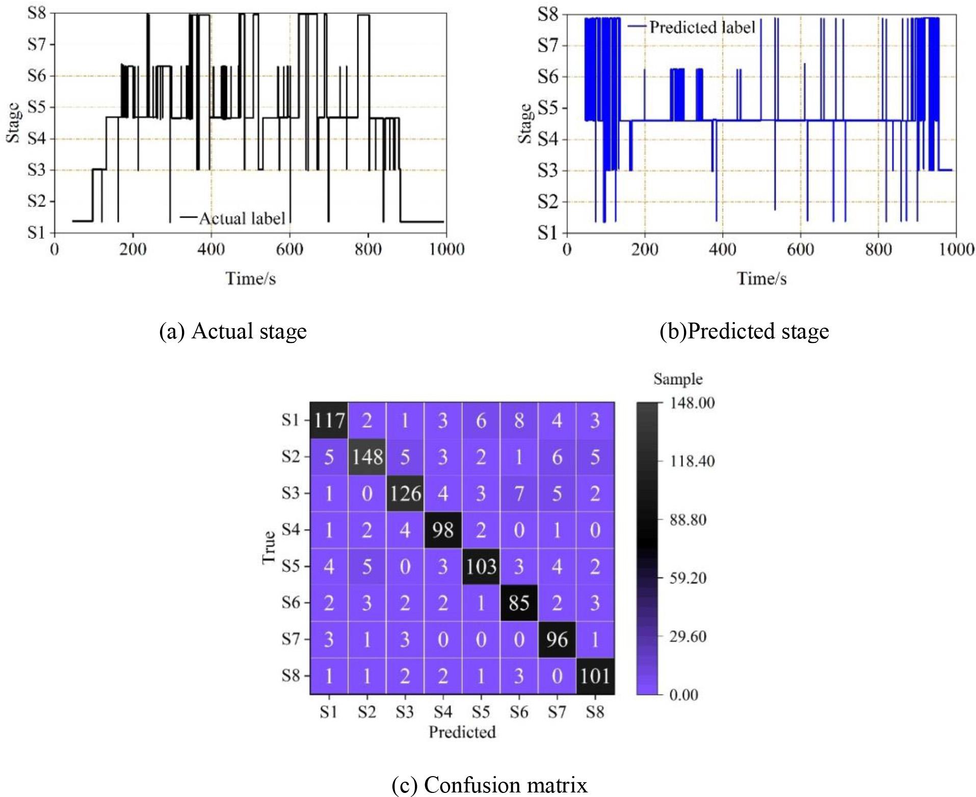
The mindfulness meditation state and the confusion matrix display of test 1
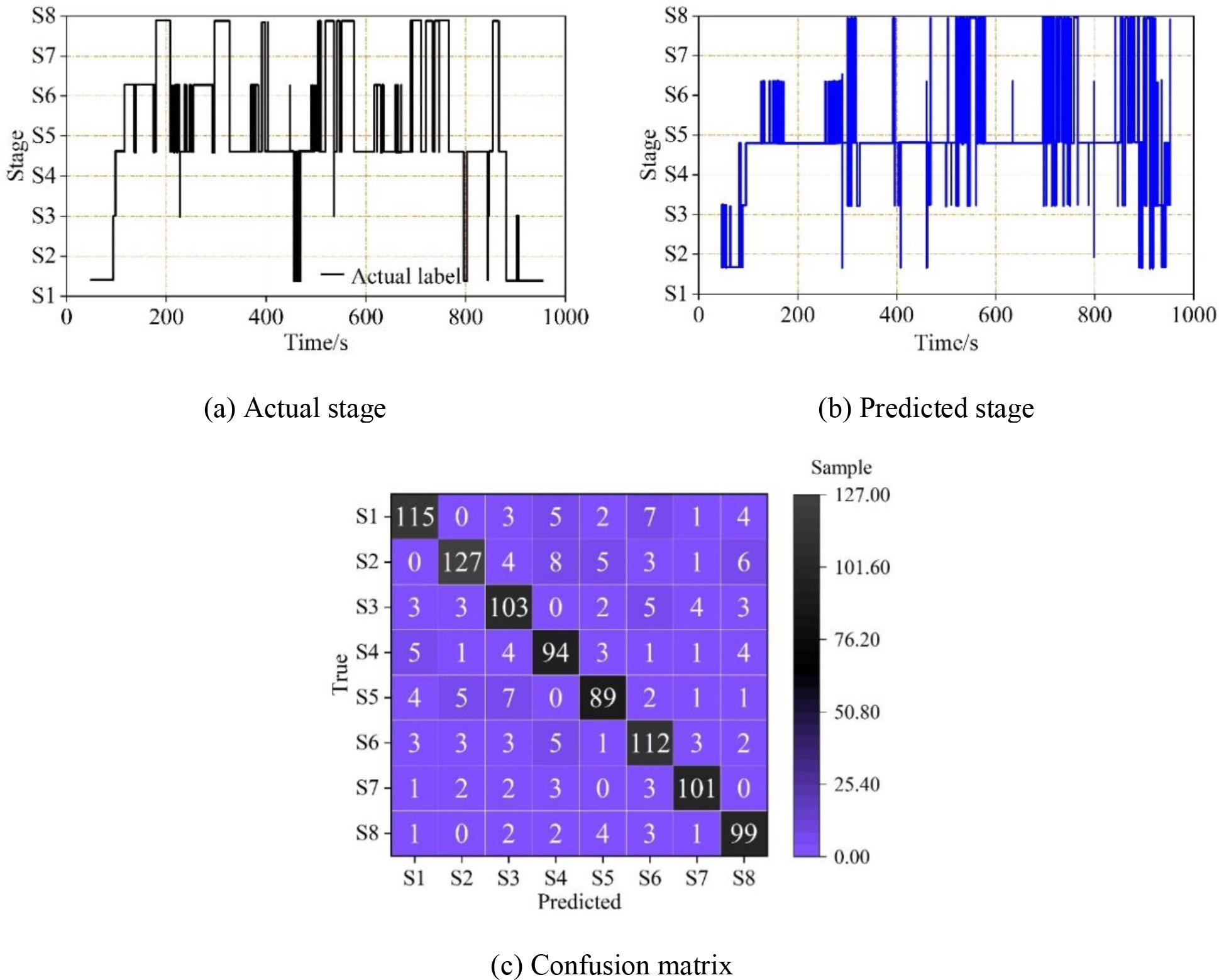
The mindfulness meditation state and the confusion matrix display of test 32
Data augmentation is a technique in the field of machine learning that aims to increase the diversity and richness of data by applying a series of transformations and expansions to the original data in order to improve the generalisation and performance of the model. The purpose of data augmentation is to simulate data changes under different conditions in the real world so that the model is better adapted to various situations.
The data enhancement method used in the study is cyclic displacement. The sampling rate of the biosignal dataset was set at 250 Hz, and with a 20s time segmentation each segment has 5000 sampling points. Assuming that the cyclic displacement is set to 250, the last 200 points of a segment are moved to the front end of the splicing, and the cycle repeats itself to increase the diversity of the data. Data enhancement was performed on the biosignal dataset, and Table 2 shows a comparison of the classification effect of the dataset before and after the enhancement for the positive thinking meditation phase. From the data in the table, after using the data enhancement method, the dataset has three enhancements in the model and the classification accuracy in the positive thought meditation stage after data enhancement is up to 91.00%. It can be seen that the data enhancement method of cyclic displacement increases the diversity of the data, as the model can extract more and richer data information features to improve the classification accuracy.
The classification effect of data enhancement
| Before | After | ||
| Evaluation index | ACC | 0.73 | 0.91 |
| Kappa | 0.62 | 0.89 | |
| MF1 | 0.68 | 0.87 | |
| F1 values per class | S1 | 0.71 | 0.83 |
| S2 | 0.66 | 0.86 | |
| S3 | 0.64 | 0.89 | |
| S4 | 0.69 | 0.84 | |
| S5 | 0.67 | 0.85 | |
| S6 | 0.63 | 0.82 | |
| S7 | 0.61 | 0.83 | |
| S8 | 0.65 | 0.81 | |
| REM | 0.71 | 0.84 | |
Due to the lack of high-quality, manually labelled biosignal data, it is difficult to satisfy the training demand of deep learning models on large-scale labelled data, and in this context, it is not only costly but also time-consuming to expand biosignal data by using traditional data augmentation methods. Compared with data augmentation, transfer learning can further effectively solve the problem of data shortage by transferring model knowledge pre-trained on a data-rich original task to the target task of frontal meditation stage classification, thus achieving model training and optimisation with a limited number of samples.
In this section, the migration learning and MobileNetV2 network model, the migration learning and ResNet50 network model, and the migration learning and Xception network model are integrated through a weighted average integration learning method to form a migration learning based integrated network for the positive thought meditation classification model. The model, i.e., Positive Thought Meditation Classification Model based on Migration Learning and Integrated Networks, is integrated to have a stronger generalisation ability than a single classification model.
The individual classification model with the best predictive performance is obtained by optimizing the training model. The predicted value of the positivity meditation classification model is obtained through the weighted average method, and then the error between the true value and the predicted value is calculated using the objective function, and then the weights are adaptively updated through the gradient descent and back-propagation algorithms to obtain the final positivity meditation predicted value. The specific process is as follows: first, pre-train the three classification models separately to achieve the best prediction performance. Then, the pre-trained models are used to obtain different predicted values, assuming that the predicted values obtained by these three classification models are
Where,
The error between the true value and the predicted value is calculated using the cross-entropy loss function:
where
Next, the backpropagation algorithm, using the gradient descent algorithm, adaptively updates the weight bar of the output values of each single classification model until the error between the output and predicted values of the integrated positive mindfulness meditation classification model is stabilised.
The study uses the stochastic gradient descent optimisation algorithm for model optimisation, with the initial learning rate of the cross-entropy loss function set to 0.003 and the number of iterations epoch set to 1000, where the Batch Size of each iteration is set to 15, and the validation frequency is set to 20. In addition, in order to prevent overfitting, a discard layer is used, where the final discard layer in the network is replaced with a probability of 0.5 for the Discard Layer.
In this experiment, the data-enhanced biosignal data of the subjects were divided into training and validation sets with a ratio of 60%. After analysing and validating the model, the parameters were adjusted, and it was confirmed after several experiments that the model had the best classification effect when the Batch Size was set to 15 at each iteration.
The number of iterations is set to 1000, and as the number of iterations increases, the classification accuracy of the model increases. Fig. 8 shows the results of the accuracy and loss value of the integrated network model for migration learning on the dataset, Fig. 8(a) shows the accuracy of the model on the training and validation sets, and Fig. 8(b) shows the loss value of the model on the training and validation sets. From the figure, it can be seen that with the number of iterations up to 1000 times, the model’s classification accuracy of positive thinking meditation on the training set is as high as 99.40%, which is a significant improvement compared to the original deep learning model and the data-enhanced deep learning model, and it can achieve an effective classification of the various stages of positive thinking meditation.
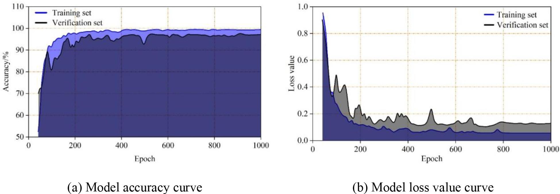
The classification effect of the model on the data set
Based on the subject’s biosignal dataset, an integrated network model based on transfer learning was applied to classify the positive thinking meditation stages as recognition, and the model was compared and analysed with GoogleNet, partial least squares discriminant analysis, SVM, random forests, BP neural networks, and the deep learning model used in the previous section. The results of the performance comparison of several models are shown in Table 3. The integrated network model performed well on the biosignal dataset with 99.40% accuracy, 93.10% recall, 87.40% Kappa index, and 95.70% F1 value. Compared to the deep learning model used in the previous section, the improvement is 8.4%, 7.4%, 7.4%, and 4.3%, respectively. It indicates that the integrated network model has significant enhancement and optimization over the deep learning model, and can more effectively achieve classification and identification of the stages of positive thinking meditation.
Performance comparison of different models
| Model | ACC | R | Kappa | F1 |
| GoogleNet | 0.914 | 0.853 | 0.732 | 0.802 |
| PLS-DA | 0.923 | 0.864 | 0.748 | 0.831 |
| SVM | 0.936 | 0.831 | 0.751 | 0.879 |
| Random forest | 0.945 | 0.879 | 0.769 | 0.893 |
| BP | 0.962 | 0.842 | 0.798 | 0.905 |
| Depth learning | 0.910 | 0.857 | 0.803 | 0.914 |
| Integrated network | 0.994 | 0.931 | 0.874 | 0.957 |
In this paper, we collect bio-signal data from subjects and process it based on the positive thinking meditation experiment. The deep learning algorithm and the long- and short-term memory neural network model are used to construct the stage classification recognition model of positive thinking meditation, and the data enhancement method is used to improve the problem of uneven data distribution in the experiment. The integration of a network model based on migration learning effectively optimizes the deep learning model’s defects in large-scale data labeling, thereby improving the accuracy of stage classification recognition in positive thinking meditation.
The deep learning algorithm combined with the long and short-term neural network classification model of positive thinking meditation has a better effect on the recognition of the data of subject 1 and subject 32, and the accuracy of the recognition of the five phases, such as resting and perceiving breathing, can reach more than 90%, but there is a problem of misrecognising the S2 phase as the S4 phase in the data of subject 32. The data enhancement method solved the problem of data inhomogeneity, resulting in a classification accuracy of 91.00% after the enhancement, an 18.00% increase from the initial results. It indicates that the data enhancement method of cyclic displacement can effectively solve the problem of uneven data distribution, thus significantly improving the classification accuracy of the model. After further optimization of the deep learning model by the integrated network model based on migration learning, the accuracy, recall, Kappa index, and F1 value on the biosignal dataset are 99.40%, 93.10%, 87.40%, and 95.70%, respectively, which are improved by 8.4%, 7.4%, 7.4%, and 4.3%, respectively, compared with the deep learning model. It further improves the stage classification recognition effect of positive thinking meditation and provides reference and guidance for optimizing the arrangement of positive thinking meditation training strategies.