AI-driven resource scheduling optimisation model and its system architecture design for digital library management

Online veröffentlicht: 17. März 2025
Eingereicht: 22. Okt. 2024
Akzeptiert: 30. Jan. 2025
DOI: https://doi.org/10.2478/amns-2025-0156
Schlüsselwörter
© 2025 Yu Zhao et al., published by Sciendo
This work is licensed under the Creative Commons Attribution 4.0 International License.
Under the premise that China attaches great importance to the concept of “Internet Plus”, the construction of digital libraries around the application of digital technology has become one of the directions for the innovative development of many libraries. The application of digital technology has considerable practical value. Not only can it improve the management effect of collection resources and reduce unnecessary management costs [1-4], but it also ensures that the readers in the process of accepting the library service get a good experience, from the overall level, to promote the library of social and public cultural services to perform the duties of the library in an orderly manner. Therefore, the library should form a correct understanding of the application of digital technology in its management and pay attention to [5-8] references to the application of digital technology needs to provide strong support to ensure that all types of emerging digital technology can be effectively applied to improve the efficiency and effectiveness of library management [9-11].
The digital library grid contains a large number of a wide variety of information resources, which will provide users with a variety of services, and how to coordinate and configure between these various types of information and services, just as a large number of signal base stations and other facilities are needed in the cable television network to regulate and control the cable television network [12-15], and the digital library grid also needs to have a regulation and control system between information resources and users, which is called the digital library grid information resource scheduling system. It refers to the release of the information resources required by users to the “edge” of the grid with the shortest distance from users [16-19] so that users can obtain the information resources they need nearby and accelerate the efficiency of users’ access to the digital library grid and the use of information resources, that is, content distribution.
This paper associates the ARIMA model and the LSTM model, combines the characteristics of library digitization management work resource time series, designs a decomposition-based ARIMA-LSTM resource prediction model, and realizes library digitization system resource scheduling based on load balancing. The prediction model is used as the resource prediction module of the Kubernetes platform, and the target node nodes are selected by judging the high load type of node nodes and regularly maintaining the queue of low load node nodes of each resource indicator type, which ultimately achieves the purpose of improving resource utilization and reliability. Applying the model for resource scheduling experiments verifies that it can improve load balancing.
With the continuous development of cloud computing, it has become the main way for libraries to build, deploy, and run digital platform applications. Cloud computing provides rich computing, storage, and service resources, facilitating users to rapidly deploy applications to meet business needs. The traditional monolithic architecture cannot fully utilize the on-demand allocation of resources and elastic scaling, and there is a risk of a single point of failure, which gradually highlights the limitations of cloud computing. To overcome these challenges, distributed systems have emerged. It decentralizes software, hardware, and network resources to multiple computers to achieve collaborative work and resource sharing. Unlike monolithic architectures, distributed systems split applications into independent services running on different nodes, which improves resource utilization through network communication and collaboration. With the development of information technology, application deployment has gone through several stages. In the early days, applications were run directly on physical hardware, resulting in wasted resources and inefficient management, as well as limited application portability and scalability. Later, the rise of virtualization technology made virtual machines a popular deployment method. VMs provide isolated virtual environments for applications, improve resource utilization and flexibility, allow multiple VMs to share physical hardware resources, and enhance portability and scalability. However, virtual machines still have the disadvantage of being resource-intensive and simulating the entire operating system and hardware environment, leading to poor resource utilization, especially in resource-intensive applications such as digital libraries.
Container technology is lighter and more efficient than virtualization technology. Containers are capable of encapsulating applications and their dependencies and deploying them across environments. The advantages are lightweight, rapid deployment, and isolation. Containers share the host operating system and kernel, consume fewer resources, and start up faster. Docker is a representative of container technology, providing tools for developing, deploying, and running containers. It utilizes Linux kernel features to achieve isolation, providing mechanisms for process, network, file, and user isolation to enhance application security and stability. However, Docker has security risks and isolation requirements that need to be considered for network and storage isolation. In addition, Docker lacks auto-scaling and scalability mechanisms. To solve the container management problem, container orchestration tools are needed, such as Kubernetes, which supports container management across hosts and clusters and provides auto-scaling, service discovery, load balancing, and network and storage isolation mechanisms to meet the security and isolation requirements of cloud environments. In cloud computing, high-performance servers are suitable for Kubernetes, but it is difficult to apply Kubernetes in restricted environments due to its excessive resource consumption.
Based on the above problems, this paper designs a resource scheduling algorithm based on an AI neural network, aiming to improve the multi-dimensional resource utilization and multi-task deployment efficiency in library digital resource management clusters.
ARIMA model
Differential integrated moving average autoregressive model (ARIMA) is a model that treats a time-varying data series as a random data series, constructs a model to describe it approximately, and then uses the past and present values of the data series to predict its future values [20].
Autoregressive modeling
Autoregressive modeling (AR) means that the value of the time series at the current time is equal to the value at previous times. Its model expression is:
Where
Sliding average models
The sliding average model (MA) is not a linear combination of historical values, but a linear combination of historical white noise that affects the predicted values at the current time. Its model expression is:
Where
Autoregressive sliding average models
Autoregressive sliding average model (ARMA) is a combination of AR and MA. Its model expression is:
When
Differential integration of moving average autoregressive modeling
In actual production, the time series usually has an unsteady nature. The time series analysis needs to be introduced into the different terms using the different operations will be unsteady time series into a smooth series. The model expression is:
Where
ARIMA model construction is mainly divided into four stages: data preprocessing, model identification, model validation and estimation, and model prediction, and its construction flow chart is shown in Figure 1.
ARIMA model construction flowchart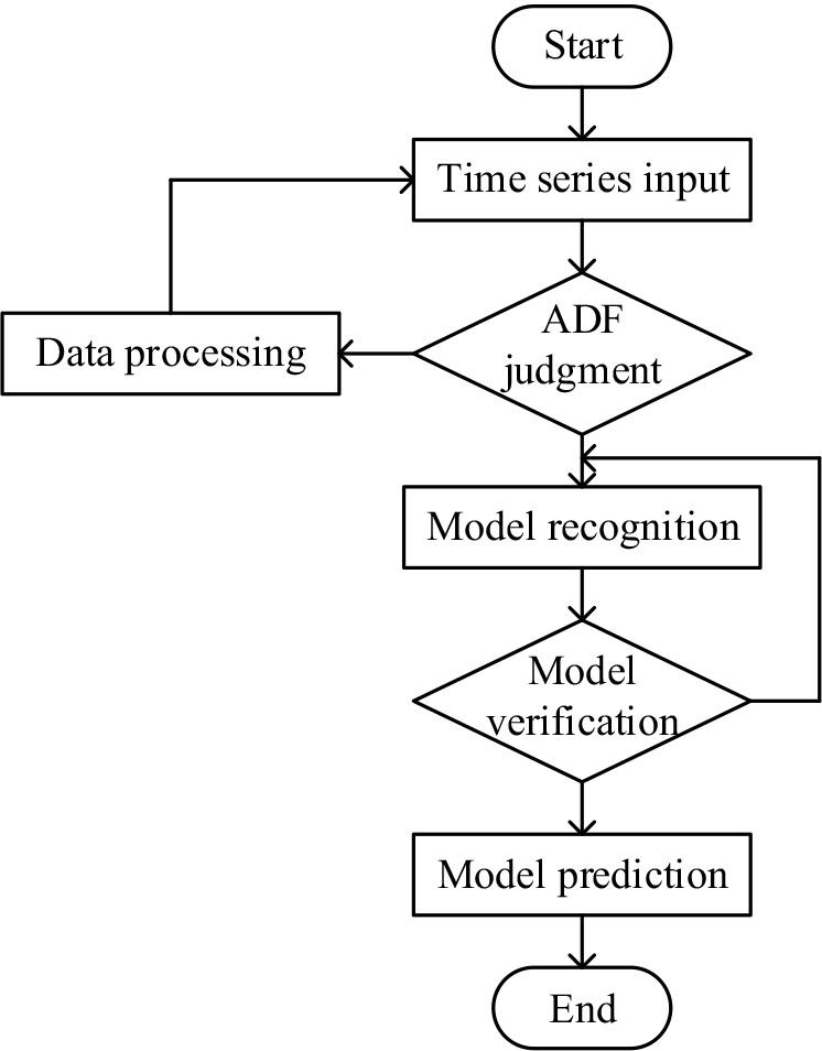
The basic characteristics of a smooth time series are twofold:
First, the time series mean is constant.
Second, the late
Where the variance of the smooth time series can be seen to be σ2.
In the model identification stage, the main task is to select the appropriate order for the model to be fitted, usually using the criterion of the minimum information criterion (AIC) so that the value that minimizes the AIC is the most appropriate model order. The AIC can be expressed as;
Gray model
GM(1, 1) is the basic prediction model of gray system theory. Constructing the GM(1, 1) prediction model first assumes that the original time series is
Combining the original time series as well as Eq. (9) yields the first-order differential equation, which is the whitening equation of the GM(1, 1) prediction model, with the following computational expression:
Where,
Where it will usually be represented as the mean series of the original time series in the GM(1, 1) forecasting model with the following computational expression:
Combining the model parameters obtained from Eq. (11), the whitening equation can be solved to obtain the time response series with the following computational expression:
The time response series are processed using a first-order cumulative series to obtain the reduced value of the GM(1, 1) prediction model with the following computational expression:
Where the expression of the generated sequence after first-order cumulative reduction of the GM(1, 1) prediction model is as follows:
Finally, the predicted values of the GM(1, 1) prediction model can be obtained according to Equation (14).
RNN model
Recurrent Neural Network (RNN) is a class of directed recursive artificial neural networks formed by connecting each neuron to itself, which are time series correlated neural networks. The RNN model computational expression is given below:
Where
RNN forward propagation
The data vector
Finally, the output sequence of the moment is obtained through the output layer of the RNN with the following computational expression:
RNN backward propagation
The backward propagation of RNN is performed by superimposing the errors caused by the gradient descent of the input and hidden layers into the final output sequence, which in turn affects the weight coefficients to be re-updated.
Long Short Neural Network (LSTM) is a recurrent neural network specialized in processing large data sequences and is suitable for medium to long time sequences and is capable of learning the correlation between before and after time [21].
LSTM is divided into three parts: forgetting, inputs and outputs, and introduces a state unit to coordinate the network.
The forgetting gate depends on the time series of the LSTM module, and the input part has the time series of the current moment, and the time series data and state of the previous moment. Its computational expression is as follows:
After the input data passes through the oblivion gate of removing invalid information, it enters the input gate, which selects and generates candidate values for the input time series, and obtains the recombined time series input data, which determines the degree of retention of the time series input data at the moment of
Where
The state unit always exists inside the LSTM and provides a state update function to update the state of the current
Selecting and updating the data at the input gate, the LSTM obtains the new time series data, and finally obtains the output data of
Where
Empirical Mode Decomposition
Empirical Mode Decomposition (EMD) is a method for processing instantaneous frequency signals. The workflow of EMD has the following four steps:
For the original time series, it is necessary to find the maximum and minimum values at each point and calculate the average value of the envelope with the expression:
Where Find the time series that satisfies the MF condition. Subtracting the IMF obtained above from the original time series is the residual series. The original time series is decomposed into multiple IMFs that satisfy the condition as well as the residual component.
Decomposition-based resource forecasting models
ARIMA and LSTM prediction models can combine the features of both models and can be used to model complex time series with higher accuracy than a single model. The specific framework of their models is shown in Figure 2.
Frame diagram of decomposed ARMI-LSTM resource prediction model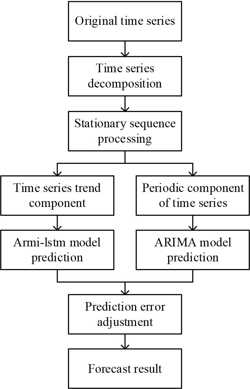
The specific steps of the decomposition-based ARIMA-LSTM resource prediction model are as follows:
The input to the resource prediction model is a continuous time series, which is represented by the following equation:
Where Training fitting of the residual value sequence using the LSTM model to obtain the trend sequence prediction value Probability estimation is carried out for the error value prediction sequence, and the data that are too large or too small in the time series are adjusted, so as to ensure the accuracy of the prediction model. Finally, the prediction results are superimposed to obtain predictions of resource utilization, and the sequence of prediction results is expressed:
The resource requirements of services are learned by the Kubernetes system beforehand. However, the default scheduling algorithm used in the current version of Kubernetes is static scheduling, which performs poorly in the changing production environment, so this paper studies and analyzes the Kubernetes resource scheduling strategy, improves and optimizes for the problems, and proposes a load balancing-based resource scheduling strategy for Pods to achieve static scheduling in a stable environment and dynamic The proposed resource scheduling strategy is based on load balancing.
The specific dynamic resource scheduling model diagram is shown in Figure 3, and the dynamic resource scheduling model is divided into a timer module, judgment module, prediction module, judgment module, selection module and migration module. The timer module is mainly responsible for periodically collecting Node node load data, periodically updating dynamic adaptive thresholds, and periodically maintaining three low load Node node queues decision module is mainly responsible for determining whether a Node node is a load Node node and determining the load type of a Node node; the prediction module is mainly responsible for predicting the future short-term load data of a Node node. The prediction module is responsible for predicting the future load data of Node nodes in the short term to avoid triggering unnecessary Pod migration due to load peaks; the selection module is responsible for selecting the Pod to be migrated among the high load Node nodes and selecting the target Node node; the migration module is responsible for migrating the Pod to be migrated to the target Node.
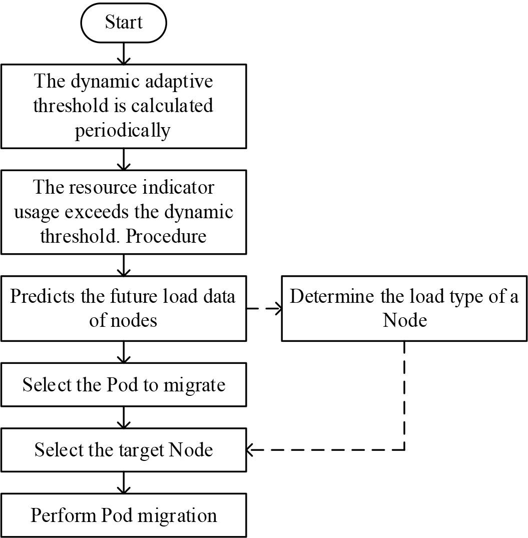
Dynamic resource scheduling process
When the utilization rate of a resource metric of a Node node has exceeded the threshold value, this indicates that the Node node is already in a high load state, and at this time, dynamic resource scheduling should be triggered to migrate some of the Pods running in this high load Node node to other low load Node nodes. If the threshold value is set too high, it will lead to some Node nodes already in high load state, but the resource utilization does not exceed the threshold value, resulting in the inability to trigger the dynamic resource scheduling; if the threshold value is set too low, it will lead to the excessive migration of Pods in the Node nodes, which will degrade the user experience and consume many unnecessary system resources. Therefore, whether the threshold size is set reasonably is particularly important.
There are two general ways to set the queue value: the static threshold approach and the dynamic adaptive threshold approach. The static queuing method is simpler to implement, but its disadvantages are also obvious. It will not change the threshold size once it is set, which will lead to the situation that if the whole cluster is in a high load state, the Pod to be migrated will not be able to find the target Node node to be placed. In this paper, the dynamic adaptive queue value will be updated periodically, while the threshold size can be dynamically adjusted according to the overall load degree of the cluster and the failure rate of Pod migration. When the overall load of the cluster is high, the threshold size will be increased; at the same time, when the failure rate of Pod migration is high, it means that it is not suitable to carry out too many Pod migrations at this time, so it is also necessary to increase the threshold size, similar to the negative feedback mechanism in biology. Mechanism.
Taking CPU utilization as an example, the calculation of other resource metrics thresholds is the same as the calculation of CPU thresholds. The following is to introduce the calculation of thresholds in detail. Setting the threshold triggered by high CPU-type load as
The formula for the value AA of the cubic exponential smoothing method is shown in Eq. (31) to Eq. (33):
The formula for calculating the value of the cubic exponential smoothing method is shown in Eq. (31) to Eq. (33)
Where:
The smoothing coefficient
In order to better place the Pods to be migrated, this chapter categorizes the high-load Node nodes into CPU-type high-load Node nodes, memory-type high-load Node nodes, and network bandwidth-type high-load Node nodes. For the same Node node, multiple resource metrics may show high load status, and then we need to distinguish which type of high load Node node the Node node belongs to according to certain rules [22]. Taking the example of both CPU and memory resource indicators displaying a high load state, the specific rules are as follows:
Calculate the load degree of the resource indicator according to the utilization rate of the resource indicator and the corresponding threshold value of the resource indicator. Taking CPU as an example, the calculation formula is shown below:
Where Compare the load degree of the two resource metrics, CPU and memory, and select the resource metric with a greater load degree as the high load type of this Node node. For example, when the load degree of the CPU is greater than the load degree of memory as calculated by the above formula, then the Node node is a CPU-type load Node node.
For the selection of Pods to be migrated, the load of Node nodes should be reduced as much as possible in a large and even manner. For example, the utilization rate of both CPU and memory resource indicators of a Node node exceeds the set threshold, and the Node node is a CPU-type Node node with a high load, if at this time, the Pods are sorted from largest to smallest according to the utilization rate of the CPU and then migrate the Pods in sequence until the CPU utilization rate of the Node node falls below the set threshold, but at this time, the utilization rate of memory resource indicators may still exceed the set threshold. Migrate the Pods until the CPU utilization rate of the Node node is lower than the set threshold, but at this time, the utilization rate of the memory resource index may still exceed the set threshold, and if the migration is performed according to the memory resource index, the efficiency of Pod migration will be greatly reduced.
The specific rule for calculating the degree of contribution W of Pod is shown in equation (37):
Where
Where
In this paper, the target Node node is selected based on the high load type of the source Node node where the Pod to be migrated is located. Three low load queues are maintained regularly, namely, CPU-type low load queue, memory-type low load queue, and network bandwidth-type low load queue. Taking the CPU-type low load queue as an example, an ordered list of CPU-type low load Node nodes is obtained by sorting all the Node nodes according to the CPU utilization rate from smallest to largest, and then excluding the Node nodes whose overall load degree is greater than the average overall load degree of all the Node nodes in the cluster. While selecting the target Node node for the Pod in the CPU-based high load Node node, the Node node at the top of the ordered list of CPU-based low load Node nodes is selected as the target Node node to be migrated [23]. In this, the overall load balancing degree LB of the Node nodes and the average overall load degree
The AI neural network-based resource scheduling model constructed in this paper is tested to examine whether its performance meets the design expectations. Static scheduling in a stable environment and dynamic scheduling in a changing environment are tested respectively to verify the prediction level and load balancing capability of the model.
In order to verify the practicality and reliability of the resource prediction and load balancing strategy of this paper, this paper builds a Kubernetes cluster in Linu, where the cluster version is 1.15, and the cluster consists of 1 master node and 4 Node nodes used for loading Pods.
Where the Pod task corresponds to a common WEB application request on the server, which is developed by using the SSM framework, when the program receives a request for a task, it writes characters and numbers through character stream related operations and then stores them in a corresponding file and returns them to the client. Afterward, the WEB application is packaged as a Docker image, and the Kubernetes cluster deploys the Pod phase to the Node worker node through a resource scheduling policy based on YAML commands. When the Pod task is deployed on the Node node, it will select a more suitable Node node for each Pod task through a series of pre-selection preferences as well as a scoring mechanism, and fully The resources of the node are utilized.
In order to observe the trend of the whole experiment, the number of Pod tasks is designed to increase linearly from 5 to 50 in step 5. When a new round of scheduling is performed, the cluster calculates the difference in the deployment time of each schedule by deleting all the Pod tasks created in the previous scheduling.
In this resource scheduling experiment, the monitoring module designed in this paper is used to monitor the utilization of various types of resources and scheduling time of the deployed Node working nodes, and a comparison of the utilization rates of various types of resources of the Node is shown in Fig. 4. Where (a) to (d) are Node1, Node2, Node3 and Node4 nodes respectively.
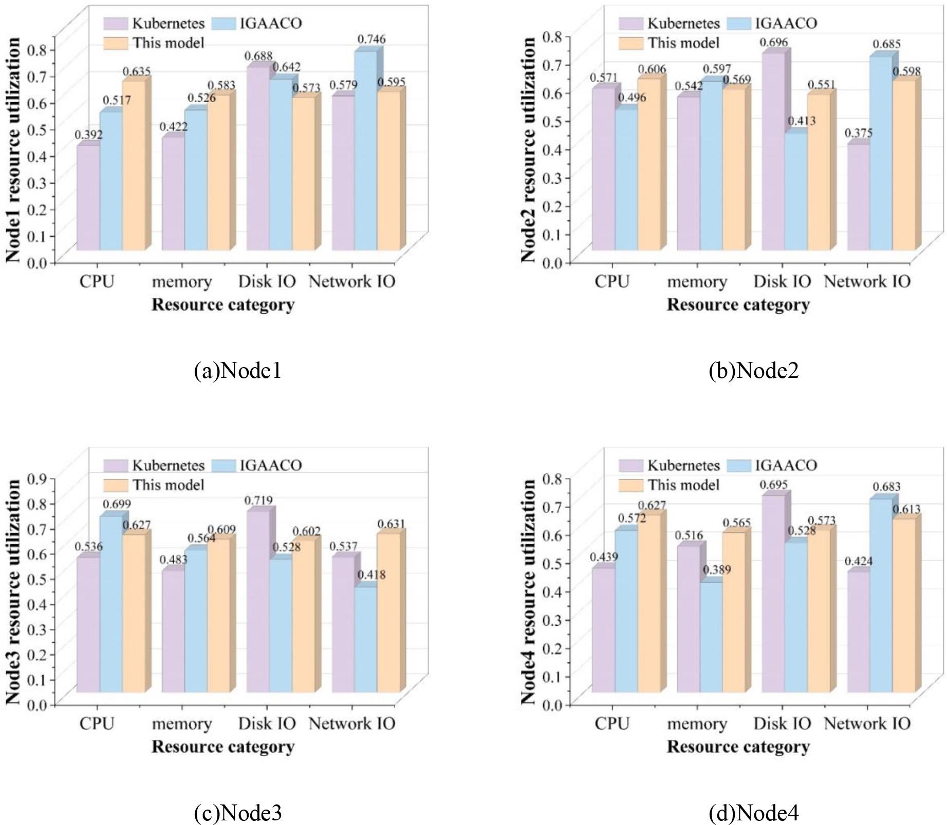
Compare the node resource utilization ratio
In the experiment for load balancing degree comparison, we compare three scheduling strategies: the Kubernetes default resource scheduling strategy, the IGAACO resource scheduling strategy based on an improved genetic algorithm, and the neural network resource scheduling strategy proposed in this paper. According to the figure, it can be seen that in the comparison of the experimental results of the resource utilization of each Node node, the Kubernetes default resource scheduling strategy has unevenly high and low overall utilization of CPU and memory in the Node1~Node4 nodes. Although the resource scheduling strategy based on the IGAACO algorithm is slightly better in the overall utilization of various types of resources, there is still a difference in the utilization of certain resources of different nodes that is too high. In contrast, the resource scheduling model that utilizes the neural network algorithm in this paper balances the load of each node in the cluster and improves its load capacity.
Also, in this experiment, the scheduling times of the three scheduling strategies for different numbers of Pod tasks in the cluster are compared, and the respective changes are plotted. The specific changes are shown in Figure 5.
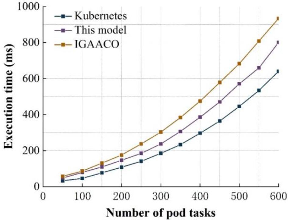
Time consumption contrast diagram
From the figure, it can be seen that as the number of pods increases, the scheduling time shows a gradual upward trend. However, the overall scheduling time is shorter due to the relative simplicity of the Kubernetes default scheduling policy algorithm. The resource scheduling time of the IGAACO algorithm and the model in this paper is relatively close when the number of Pod tasks is small, but the scheduling time gap increases as the number of Pod tasks keeps increasing. In the case of an increasing number of pod tasks, the model presented in this paper requires less scheduling time.
The dynamic network scenario experiments are performed next. The settings for dynamic resource scheduling triggers are as follows:
The system is initialized, and parameters such as system resource specification factor, demand weight factor, dynamic scheduling threshold, and load information collection period are set. The 0Kubelet component obtains the load information of each working node at regular intervals according to the set period, which is generally set to 20-60 seconds, and stores the collected load information into the etcd database. The master node reads the load information from the etcd database and obtains the scheduling scheme under the dynamic scenario according to the strategy of dynamic load balancing and delay optimization. The scheduler completes the migration of Pods and access requests and assigns them to the specified Node according to the scheduling scheme.
On a small scale, three simulation experiments were also designed with three different total access scales. In all three types of simulation experiments, the number of nodes is set to three, and the number of pod types that need to be deployed in total each time is set to four.
A comparison of the load balancing degree and delay condition of the three simulation results under the small-scale dynamic scenario is shown in Fig. 6 and Fig. 7.
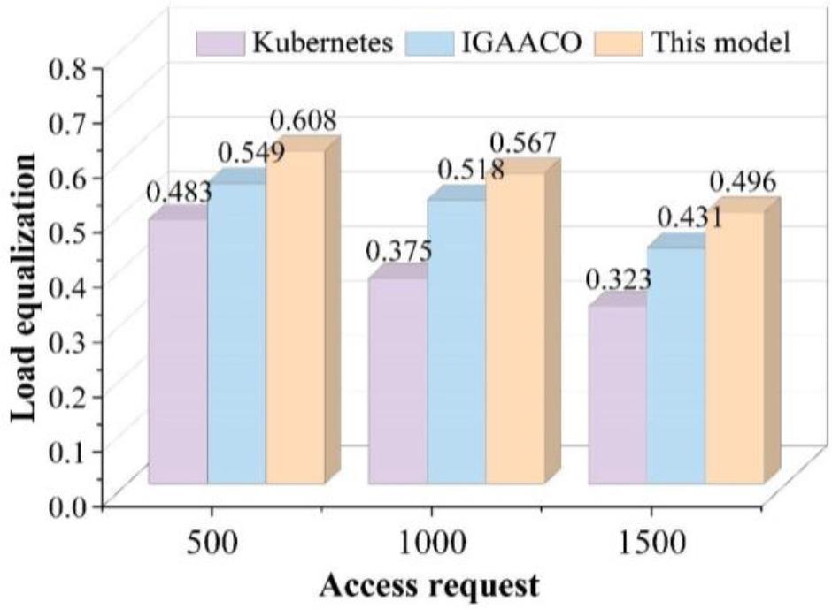
Dynamic small-scale simulation load equalization
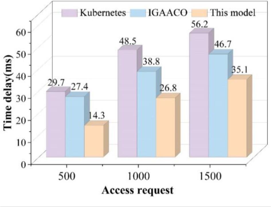
Dynamic small-scale simulation of delay changes
A load balance of 1 means that each node in the cluster has the same utilization rate of CPU and memory resources, and the cluster is optimally loaded, and vice versa. The lower the value of load balance means that the resources are unevenly distributed among the nodes in the cluster. From Fig. 6, it can be learned that the resource load balancing status of the cluster is very low before Pod performs dynamic migration, and after the redeployment of the dynamic scheduling model, the resource load balancing of the cluster significantly rises and is slightly better than the dynamic migration scheme of the IGAACO algorithm. From Fig. 7, it can be learned that due to the increasing number of accesses, the overall delay of the cluster is also at a high level, and after the accesses are re-shifted and re-allocated by the dynamic scheduling model, the overall delay of the cluster has been reduced to a certain extent, and the overall reduction of this paper’s model is better than that of the IGAACO algorithm.
In this paper, we design a decomposition-based ARIMA-LSTM resource prediction model and implement resource scheduling for library digitization systems based on load balancing. Static and dynamic scheduling experiments were conducted, and it was found that Kubernete’s default resource scheduling strategy has high and low overall CPU and memory utilization in Node1 to Node4 nodes. Although the resource scheduling strategy based on the IGAACO algorithm has a slightly better overall utilization of all types of resources, there is still a significant difference in the utilization of certain resources in different nodes. In contrast, the resource scheduling model based on the neural network algorithm in this paper can make the load of each node of the cluster more balanced and improve the load capacity of the cluster. After the dynamic scheduling model reallocates accesses, the overall latency of the cluster is reduced, and this paper’s model achieves a better overall reduction than the IGAACO algorithm.