Deep Learning Based Fault Detection and Diagnosis Method for Power Systems

Published Online: Mar 17, 2025
Received: Oct 11, 2024
Accepted: Jan 29, 2025
DOI: https://doi.org/10.2478/amns-2025-0200
Keywords
© 2025 Gaoyu Lin et al., published by Sciendo
This work is licensed under the Creative Commons Attribution 4.0 International License.
Power system is one of the infrastructures of modern industry and life. However, due to the complexity of the system and the variability of the operating environment, power system failures are inevitable. The occurrence of faults may lead to serious consequences such as power outage, equipment damage, and even fire. Therefore, the research and application of power system fault detection and diagnosis methods have become particularly important [1-4].
The current fault detection methods include insulation diagnostic technology, cable diagnosis, infrared scanning image and so on. At present, certain progress has been made in power system fault detection and diagnosis methods. However, there are still some challenges and problems to be solved [5-8]. First, the types and modes of power system faults are very complex and diverse, and different types of faults may require different detection and diagnosis methods. Therefore, how to select and design appropriate methods for detecting and diagnosing different types of faults is an important issue [9-11]. Secondly, the process of power system fault occurrence and propagation involves multiple devices and systems, and the data acquisition and processing face great challenges. How to improve the efficiency of data acquisition and processing, and ensure the reliability and accuracy of data is an urgent problem [12-15]. In addition, fault detection and diagnosis methods for power systems need to be combined with power system operation and maintenance to form an integrated solution [16-17].
Literature [18] describes the application of fault diagnosis techniques to power systems, including pattern recognition techniques and unsupervised quarter-sphere support vector machine techniques, with a focus on reliable detection and classification of power system faults. Literature [19] reviewed fault diagnosis methods for power transmission systems, classifying and localizing faults through the use of artificial intelligence and signal processing, and comparing various methods of fault detection, classification and localization. Literature [20] outlines the types and causes of faults in PV systems and analyzes current fault diagnosis methods, especially for faults occurring in PV arrays. The advantages and limitations exhibited by FDD methods in terms of complexity and cost-effectiveness of large-scale integration are shown. Literature [21] emphasizes the important role of FDD for power systems. Literature published from 1990 to 2020 is categorized to provide a systematic discussion of FDD techniques and algorithms based on different viewpoints. The advantages and disadvantages of current fault detection and diagnosis methods are also summarized to lay the foundation for subsequent research. Literature [22] reviewed machine learning for power system fault diagnosis. It introduces the application, framework and workflow of machine learning in power system fault diagnosis, and discusses the unsupervised and supervised learning techniques, and analyzes the advantages and disadvantages of various diagnostic techniques. Literature [23] discusses the application of intelligent systems in power system transmission line fault diagnosis, and summarizes the classification of the strategies used and the relationship between the techniques through a literature review to identify the development trends associated with intelligent fault diagnosis systems for transmission lines. Literature [24] explores the application of artificial neural networks in detecting, classifying and localizing faults in power systems. The wscc9 bus test system is modeled and the proposed detection system is validated. It was shown through fault simulation that the output of the artificial neural network should provide information about the type and location of the fault when it occurs.
Literature [25] explains the application of machine learning in fault diagnosis. It was emphasized that power systems are becoming flexible and complex and hence it is necessary to improve fault diagnosis techniques in power systems to prevent damage from fault occurrence. Literature [26] after reviewing the literature related to fault detection in PESs proposed techniques of data mining including machine learning, deep learning algorithms, etc. and by introducing signal measurement sensors to express the fault detection procedure in PESs. The performance of various data mining techniques in fault detection is evaluated and the results show that deep learning techniques are more effective as compared to other methods. Literature [27] mentions and describes the hybrid framework that can rapidly detect and localize transmission line faults and presents the methodology for analyzing the techniques, the pattern recognition approach through neural networks and the joint decision making mechanism. Experiments verified that the hybrid framework can achieve fault detection, classification and localization in a short period of time, which effectively improves the fault clearance time. Literature [28] introduces a methodology for fault interference detection based on wavelet transform and independent component analysis (ICA), which is achieved by detaching the voltage signals from the fault state for processing and analyzing them using wavelet transform and ICA, and it is concluded through tests that the methodology shows sufficient robustness in various operating scenarios under noiseless and frequency varying conditions. Literature [29] aims to use the support vector machine method for detecting fault detection in power systems by using training data before and after faults in bus voltages, generators in order to detect system anomalies, after resolving the disturbances the support vector machine will be able to determine the state of the fault.
In this paper, a power system fault diagnosis model based on CNN-Attention-LSTM is formed using various deep learning techniques including Convolutional Neural Networks, Long and Short Term Memory Networks and Channel Attention Mechanism. The power fault information is collected and processed, and a number of power system fault detection and diagnosis evaluation indexes, such as precision rate, recall rate and F1 value, are designed to evaluate the effectiveness of the method proposed in this paper through fault detection. It shows good generalization ability for different power scenarios such as high resistance faults, cable faults and transformer faults.
The transient signal contains a large amount of information reflecting the fault characteristics, and the differences in the energy contained in different frequency components of voltage and current provide a basis for fault characterization. Power system fault detection can use the transient signals generated at the time of fault occurrence to extract the zero-sequence voltages and zero-sequence currents after the fault occurs [30].
The characteristic quantity that characterizes the fault is defined as:
The wavelet detail coefficients after wavelet processing are calculated by applying the above formulae, and the spectrum of quantities
The specific steps of the fault detection algorithm are as follows:
Step 1: Collect phase voltages
Step 2: After vector sum
Step 3: Reconstruct the associated
Step 4: Calculate the absolute value of the
Step 5: Determine the final location of the high resistance fault line through the comprehensive judgment of the above information.
The initial image with substation equipment targets is input to the network by pixels, feature extraction is performed in the convolutional layer, the pooling layer performs dimensionality reduction of the features and repeats the construction a number of times for more abstract semantic information, and finally the features are sent to the all-connected hierarchical classification for localization [31].
Convolutional layer can be used as a feature extractor, which can autonomously learn the effective features of the target image. The output at the end of the convolutional layer is called the feature map. The size of the convolution kernel and the input target feature image are 3 × 3 and 5 × 5, respectively. The convolution kernel is slid over the input target feature image with a step size of 1. In order to obtain a new target feature map, the inner product of the input target feature image and the corresponding position of the convolution kernel is calculated. The size of the output target feature image obtained after calculation is 3 × 3.
Pooling layer to start the selection of target features to first reduce the spatial size of the target feature image, through the convolutional layer of feature extraction after the output image will contain a certain degree of redundant information. Pooling layer has the effect of removing redundant information, maximizing the key feature information left, and then further feature extraction of the feature target image.
The fully-connected layer is composed of multiple hidden layers using the fully-connected method, and the nodes of each layer are linked to the nodes of the next layer according to certain weights. In addition, the input of the fully connected layer is the feature map converted into the corresponding feature vector, and the fully connected layer is combined with the pooling layer and the convolutional layer to extract the local features of the image, and then generate the overall features of the target image. The core operation of fully connected is matrix multiplication, which is calculated as follows:
Where,
The internal structure of the LSTM neural network is shown in Figure 1.
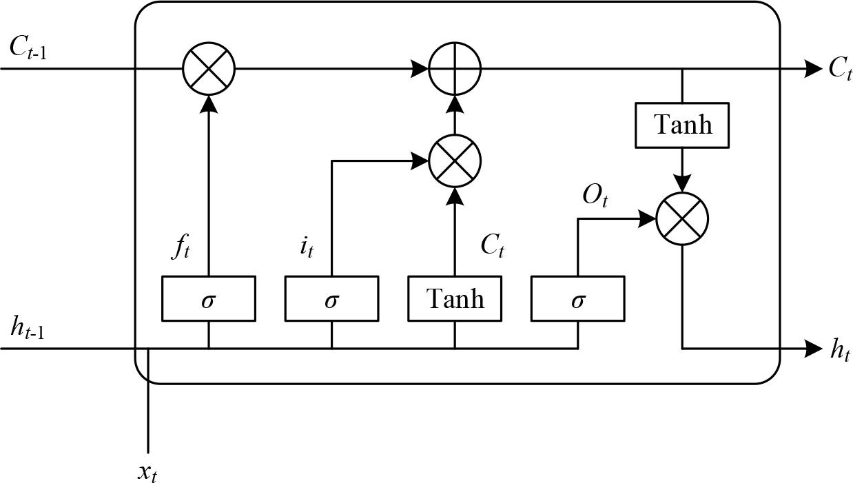
LSTM Network structure
In LSTM neural network [32], the expression of the input gate is Eq. (3), the expression of the forgetting gate is Eq. (4), Eq. (5) and Eq. (6) are the expressions for the associated state update, the expression of the output gate is Eq. (7), the expression of the hidden layer at this moment is Eq. (8), and the specific expression of the activation function is shown in Eq. (9) and Eq. (10):
Where
The attention mechanism basically consists of the following processes: firstly, the attention channel module is applied to correct the features of the input image to get the feature map
In order to enhance the computing efficiency of the channel attention module and improve the feature extraction accuracy of the input samples, this paper applies two pooling methods, GAP and GMP, to efficiently compress the spatial dimensional features of the input model, so as to obtain the channel features of the input samples Fig.
Where
The main function of the MLP module is to effectively fuse the global maximum pooling vector and the global average pooling vector, input the fused parameters into the model activation function, and finally obtain the channel attention vector, the channel attention structure is specifically shown in Figure 2.

Channel Attention Structure Diagram
In this paper, we propose a deep learning-based cable fault diagnosis model for power systems, which takes the fault raw current data as input and automatically extracts the fault features from the current signal through 1D convolution operation.CNN adaptively completes feature extraction and data dimensionality reduction through convolution and pooling operations, and has a better generalization ability than the traditional feature extraction methods.LSTM has a LSTM has unique advantages in processing long time series data. In this paper, CNN and LSTM are combined to design a branch line fault diagnosis model based on CNN-LSTM.
In this combined model, CNN introduces weight sharing through cascading in the operation process, and after maximum pooling, although the global features can be obtained through local scanning and screening, it cannot distinguish the influence of each feature on the classification results, which leads to a certain upper limit of the CNN-LSTM diagnostic model in terms of convergence speed and recognition accuracy. To solve this problem, this paper adds a channel attention mechanism after the pooling operation of this model, which screens high-level features in the channel domain by adaptively learning the correlation between the channels, and sends the data obtained after screening to LSTM for fault recognition. The overall structure of CNN-Attention-LSTM cable fault diagnosis designed in this paper is shown in Figure 3.
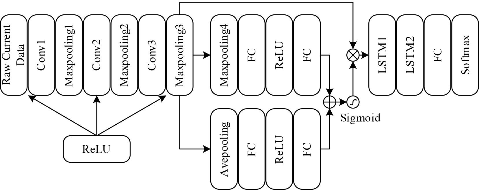
The overall structure of the CNN-Attention-LSTM fault diagnosis
By adjusting the model structure of CNN-LSTM, CAM is introduced after three layers of convolution and pooling operation, and its core idea is to realize differentiated processing through different channels, the detailed process is as follows: the features after convolution operation are respectively subjected to two different operations, maximum pooling and average pooling, and the obtained result is taken as the input of the MLP network to perform the fully-connected operation, which is weighted and summed up to output the feature weight values through the Sigmoid activation function outputs the feature weight values, and finally multiply with the original signal to output the feature results. Compared with the features extracted by the convolutional neural network for classification, the CAM can be applied to scenarios with limited computational resources to a certain extent by adaptively adjusting the feature response values.
The online diagnosis process of power system cable faults designed in this paper is shown in Figure 4. In network training, the fault sample set is first labeled and normalized, and the samples are divided into a 4:1 training set and a test set. In the adjustment phase of the model training parameters, the gap between the prediction results and the real labels is calculated using the cross-entropy loss function (CCE), and the network parameters are continuously adjusted by the BP algorithm and the Adam optimization function in order to minimize the loss function value. When the model training is completed, the network model with optimal performance is saved, and the test set is used to verify the model generalization and analyze the diagnostic results more intuitively through the confusion matrix. At the same time, the real-time monitoring data can be pre-processed and input to the trained network module to realize online fault diagnosis.
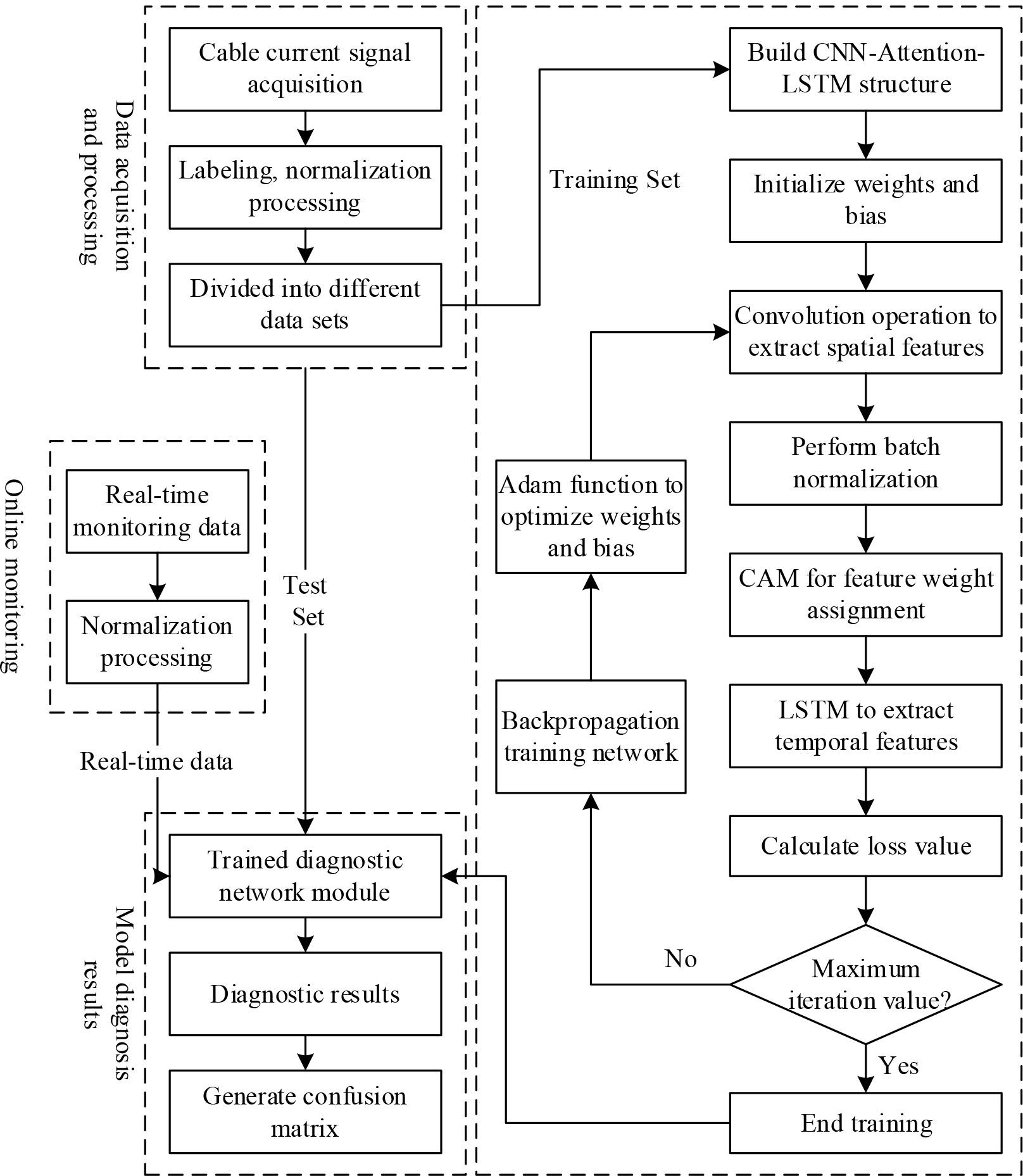
The electrical system fault online diagnosis process
The experimental data used in this paper mainly comes from a State Grid ICT company, mainly recorded in the company in the power system including cable faults and other information and fault disposal measures, the power fault data set contains 37,613 entity numbers, which consists of fault information, fault causes, fault site points, fault disposal measures of the four entity sets.
The obtained original power system fault data is preprocessed by Python, and the data is standardized by using Pandas and numpy modules, for example, there is a situation that the case format of “Minor” and “minor” is not uniform in the fault severity level. Therefore, the quality of the fault text is improved through data preprocessing, the noise data of the fault text is reduced, and the accuracy of entity recognition is improved.
In this paper, we adopt the “BIO” annotation mechanism, where B represents the first word of the entity, I represents the middle and the last word of the entity, and O represents the non-entity elements. The annotated data is exported to ann file, and then the Python code is used to transform the ann file into BIO annotation.
In this paper, the commonly used evaluation metrics in entity recognition: precision (P), recall (R) and F1 value (F1), accuracy (A), reliability (D) and security (S) are used to carry out the work of evaluating the performance of the model, which are defined in the following equation:
Where
The computer used in the experiment was configured as follows: the Windows 10 operating system, CPU model Intel(R) Xeon(R) CPU E5-2650v3@2.30GHz2.30GHz (2 processors), 64 GB of RAM, python 3.8, Tensorflow 2.5.0, gensim 3.8.3. The main parameters of the model in the experiment are configured as seq_length of 128, batch_size of 64, and learning_rate as default.
In order to test the ability of the high resistance fault detection algorithm to recognize the faulty phases of the power system, this section creates a certain scenario, chooses a total of four phases A-D, and sets a high resistance fault occurring in phase A to test the detection effect of the proposed fault detection method. Figure 5 shows the detection results of this paper’s method on the faulty phase of the power system.

Test results of failure of power system
From the data in the figure, it can be seen that the proposed method in this paper crosses the threshold value of 0.15 in about 0.3 s, and remains between 0.5 and 0.6 until the end of the 20th detection point is still above the threshold value, and the duration is more than 1.2 s. The detection folds of the three phases of B, C, and D do not appear to cross the limit, which can be determined that the A-phase faults, i.e., the A-phase grounded high-resistance faults.
In order to compare the detection performance of the proposed method with other detection methods, PCA-JSD, WP, and SWT are selected as the comparison methods in this section, and 500 groups of high-resistance fault cases and 500 groups of normal cases are randomly generated to compare the method performance by using the three performance indexes, namely accuracy (A), reliability (D), and safety (S). The three indicators are represented as follows:
The comparison results of the three evaluation indicators are shown in Fig. 6. As can be seen from the figure, the method proposed in this paper is better than the comparison method in terms of accuracy, reliability and safety, and it is 8%, 12.2% and 4.8% better than the comparison method with optimal performance (WP), respectively.
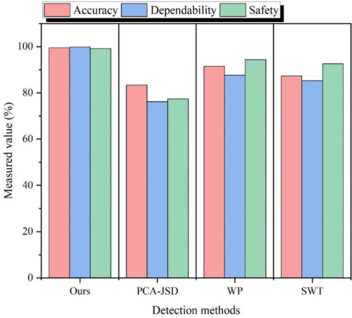
The three evaluation indicators compared the results
In order to verify the learning effect of the CNN-Attention-LSTM fault diagnosis model proposed in this paper, it is compared with CNN and LSTM, based on the training set for the overall training of the three models. The number of training rounds is 200, and the evaluation indexes are Loss, Accuracy. During the model training process, the smaller the value of the loss function, the more accurate the model prediction.
The training results of the validation set of each model are shown in Fig. 7, from which it can be seen that with the increase in the number of iterations, the loss value and accuracy of the three neural network models tend to converge. However, the CNN-Attention-LSTM model proposed in this paper is better than the comparison model in both convergence speed and convergence effect. The data show that when the training iteration reaches about 30 rounds, the Loss value and accuracy of the model in this paper converge to 0.12 and 0.94 respectively, while the comparison model needs 40 rounds to complete the convergence slowly. This indicates that the model in this paper has more power system fault diagnosis learning ability.
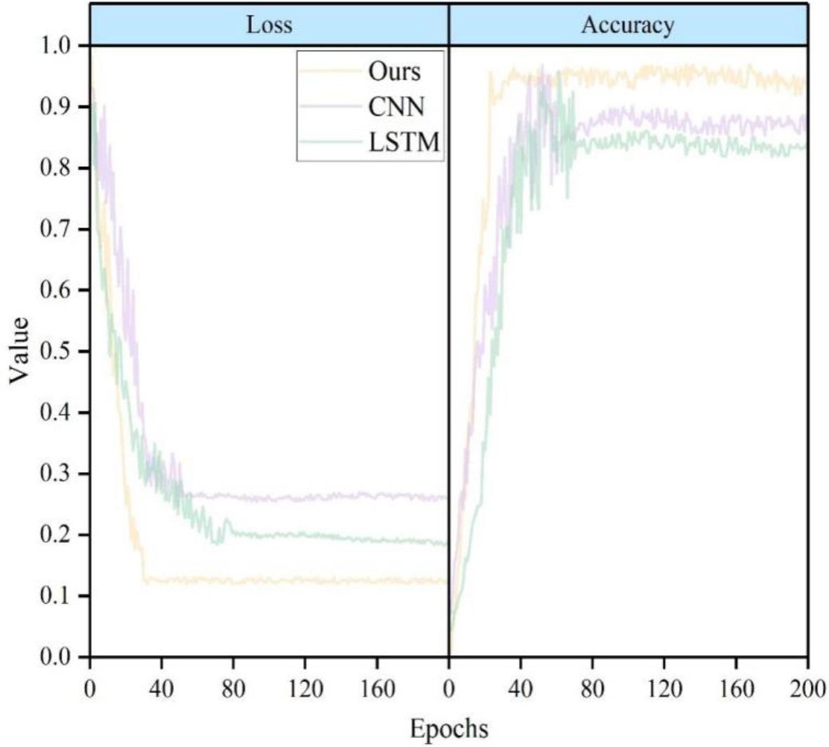
Model validation training results
In this section, CNN and LSTM models are still selected for the power system cable fault classification experiments. Accuracy (ACC), precision (P), recall (R) and F1 value are selected as model evaluation parameters, aiming to verify the performance of the CNN-Attention-LSTM prediction model proposed in this paper.
The results of the performance evaluation of different prediction models are shown in Fig. 8. According to the experimental results, the CNN-Attention-LSTM power system fault diagnosis model designed in this paper, the values of the four evaluation parameters of ACC, P, R and F1 value are stable above 96% under normal, series, parallel and hybrid cable faults, while the four evaluation parameters of the two groups of comparative models of CNN and LSTM are distributed in the range of 85% to 92%. The CNN-Attention-LSTM model designed in this paper is characterized by high stability and fast convergence compared with traditional neural networks, indicating that the fault diagnosis model in this paper can effectively classify cable faults in power systems.

Different prediction model performance evaluation results
In this section, for the transformer fault types, including short circuit faults, overload faults, overvoltage faults, undervoltage faults, grounding faults, disconnection faults, arcing faults, harmonic faults, and normal conditions, 10 kinds of faults, which are denoted as fault types 1-10 in turn. And use ADC-SVM, CS-SVM, GWO-SVM, and HGWO-SVM as the comparative models to compare the diagnostic effect of the transformer fault types with the CNN- Attention-LSTM model to compare the diagnostic effect for transformer fault types under the same operation state of the power system. In order to test the diagnostic ability of the model transformer faults in this paper, and verify its comprehensiveness in fault diagnosis. The results of the comparison of the diagnostic effect of different methods under the transformer fault state of the power system are shown in Figure 9.
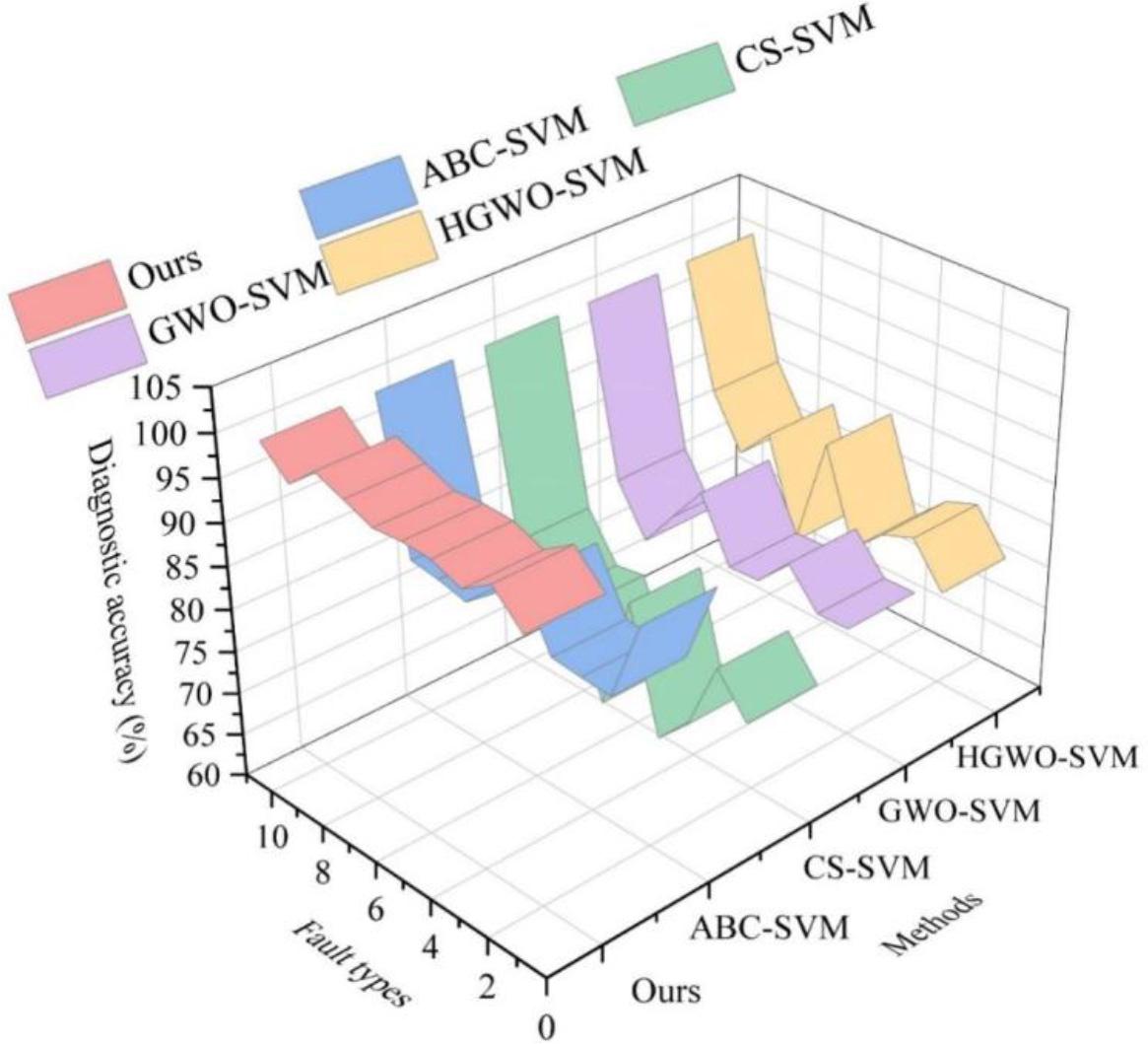
The results of the diagnostic results of different methods of the same fault
As can be seen from the figure, the diagnostic methods proposed in this section have a diagnostic accuracy of more than 95% for transformer faults, in which the harmonic faults and the data in the normal state are highly responsive, and the diagnostic accuracy is 100%, which indicates that the model constructed in this paper can dig out the effective information and has better diagnostic effect. Although the other four methods can achieve the same effect in the normal state, they perform extremely poorly in the remaining 9 faults, in which the CS-SVM method has the lowest accuracy for fault diagnosis, with an average accuracy of 72.43% for 9 fault diagnosis, indicating that the method cannot effectively identify the data information therein.
In summary, the methods proposed in this section have high diagnostic accuracy in various scenarios of power system fault problems. However, from a practical point of view, it is still necessary to pay attention to the diagnostic study of power system faults, so that the model can better identify the latent faults within the power system to ensure the safety of power supply to the grid.
In this paper, a CNN-Attention-LSTM power system fault diagnosis model based on deep learning is constructed. Through several simulation experiments, we analyze the effect of the proposed method and model in this paper. The following experimental results are obtained:
1) The high-resistance fault detection method in this paper can recognize power system fault phases beyond the threshold value, and its accuracy, reliability and security are improved by 8%, 12.2% and 4.8%, respectively, compared with the WP method. 2) The evaluation index values of this paper’s model under normal, series, parallel, and mixed cable faults are all greater than 96%, indicating that it can accurately classify cable faults. 3) The diagnostic accuracy of the model in this section for common transformer faults is still up to more than 95%, and the diagnostic accuracy for harmonic faults and normal condition is 100%.