Application of high-precision three-dimensional mapping technology in urban housing structural safety inspection

High-quality development has become a trend in the development of all industries in China. After decades of development, China’s residential construction has changed from a simple quantity expansion stage to a quality improvement stage. With the progress of society and the improvement of people’s living standards, the people’s demand for living in existing residences has gradually increased, and their demand for the quality of existing residences has become higher and higher [1-3]. China has a huge number of existing residences, however, some existing residences have outstanding structural safety problems, which can not meet the residents’ living needs [4-5]. In order to comply with the development trend of high quality in the new era, improve the degree of satisfaction of the residents’ living demand for existing houses, and enhance the quality of existing houses, it is urgent to make accurate and scientific testing of the structural safety of existing houses.

Most of the traditional housing safety appraisal methods rely on manual regular observation and measurement, which are time-consuming and laborious, difficult to meet the needs of housing safety monitoring, lack of integrated management, and unable to achieve real-time dynamic monitoring of old houses [6-8]. The analysis and mapping work is the most effective means to understand and transform nature and is also one of the works with strong basicity, preliminaries and advancement, which is an indispensable work link in urban planning and management [9-11]. Various data, maps and other products produced by three-dimensional mapping technology can be utilized to provide information services and theoretical basis for various stages of planning and management [12-13]. High-precision urban three-dimensional mapping data can intuitively respond to the urban landscape, which covers almost all the information about geographic features, cadastral properties, etc., which are the basis for the planning and management of a city [14-17]. The use of urban three-dimensional mapping technology to detect the structure of urban housing can be in the protection of the owner’s safety under the premise of the safe use of the building, to avoid all kinds of building collapse accidents, extending the service life of the house, to promote the harmonious progress of the society, for the future standardization of the development of the house building to provide a security guarantee [18-21].

Based on the theoretical model of ranging accuracy, this paper proposes the streak array detection LiDAR mapping technology, which calculates the target distance and confirms the ranging transfer error value through the centre of mass weight method. Using the striped array 3D detection technology, the target housing is scanned in broom style, and the distance image of the target on the ground is deduced based on the inertial navigation system and the distance inverse algorithm. After indexing the scan lines, the striped array detection technique is used to retain the bump features on the walls of the housing building. The RANSAC algorithm, combined with the eigenvalue method, is used to perform automated feature extraction and plane fitting on the 3D point cloud data to detect the structural safety of the urban housing structure in terms of dimensions, flatness, and perpendicularity. The test results and the prediction results are analysed empirically, and the measures for the management of housing structure settlement are proposed through the finite element analysis method, and the prediction results of the management of the measures are analysed.

2

Structural safety testing of urban housing

2.1

Theoretical model of ranging accuracy

2.1.1

Stripe Array Detection Lidar Ranging Accuracy

Stripe array detection lidar usually has 1000~2000 sampling channels, and each laser pulse can obtain a large number of echo signals. Since the stripe array detection lidar system has multiple sampling channels, the system’s root mean square error (RMSE) can be calculated by imaging a planar target in a practical measurement, and the RMSE value can be derived from the following formula: (1) $Δ_{r a n g e} = {[\frac{1}{N} \sum_{i = 1}^{N} {(R_{i} - R_{f i t, i})}^{2}]}^{1 / 2}$ Where R_i is the result of distance calculation for the ind sampling channel (m) and R_frij is the corresponding distance value of the fitting result in the ith sampling channel (m).

2.1.2

Three main types of errors in striped array detection lidar

Stripe array detection lidar systems contain three main types of ranging errors: additive noise-induced errors, multiplicative noise-induced errors, and sampling errors, and the total ranging error of the system is the result of the combined effect of the three main types of errors [22]. The error caused by noise is due to the signal strength being interfered with by noise and not being able to reproduce the original waveform, while the sampling error is due to the fact that the CCD has a certain pixel size, and the echo signals within each sampling channel produce a grey scale homogenisation effect. The additive noise of the system is a noise independent of the signal strength, while the multiplicative noise of the system has a positive relationship with the signal strength, so the ranging error caused by the two types of noise should be independent of each other. Sampling error, also known as algorithm error, which mainly depends on the sampling frequency and signal identification algorithm, is a kind of error independent of the noise intensity. Therefore, the three main types of errors of the system are independent of each other, and the total ranging rms error of the streak array detection lidar can be expressed as: (2) $Δ_{r a n g e} = \sqrt{Δ_{a d d}^{2} + Δ_{m u l}^{2} + Δ_{s a m p l e}^{2}}$ Where Δ_add is the ranging error due to additive noise (m), Δ_mul is the ranging error due to multiplicative noise (m), Δ_sample is the sampling error (m).

2.1.3

Ranging error transfer

Centre of mass weighting (COG) is a method of determining the distance to the target by calculating the position of the centre of mass of the signal distribution using the formula [23]: (3) $R_{c a l} = \frac{\sum_{i = 1}^{N} r_{i} I_{i}}{\sum_{i = 1}^{N} I_{i}}$ Where R_cal is the calculated target distance (m), I_i is the grey scale value of the signal strength of the ith sampling point, r_i is the distance coordinate value of the ith sampling point (m).

This algorithm has very good robustness, at the same time, due to the full use of the signal strength of each sampling point to judge the final target distance, which can take into account the calculation accuracy on the basis of guaranteeing the calculation speed Therefore, the COG algorithm has been widely used in the signal discrimination process of the streak array detection LIDAR, and this paper will also be based on this algorithm to establish a theoretical model of the system’s ranging accuracy.

Using the centre-of-mass weighting algorithm described in the previous section, the centre-of-mass position x_cal of the signal can be determined from the signal strength I_i of the sampling point and the coordinate value x_i of the sampling point: (4) $x_{c a l} = \frac{\sum_{i = 1}^{N} x_{i} I_{i}}{\sum_{i = 1}^{N} I_{i}}$

In turn, the calculated distance to the target is determined by combining the time slot width and the distance from gate start distance values: (5) $R = \frac{x_{c a l} t_{b i n} c}{2} + G a t e_{1}$

To facilitate the derivation of the formula order: (6) ${\begin{array}{l} u = \sum_{i = 1}^{N} x_{i} I_{i} \\ v = \sum_{i = 1}^{N} I_{i} \\ w = \sum_{i = 1}^{N} x_{i}^{2} I_{i} \end{array}$

Then Eq. (4) can be simplified as: (7) $x_{c a l} = \frac{\sum_{i = 1}^{N} x_{i} I_{i}}{\sum_{i = 1}^{N} I_{i}} = \frac{u}{v}$

According to the basic theory of error transfer, the error in the position of the centre of mass can be obtained as: (8) $\begin{matrix} σ_{x}^{2} = σ_{u}^{2} {(\frac{\partial x_{c a l}}{\partial u})}^{2} + σ_{v}^{2} {(\frac{\partial x_{c a l}}{\partial v})}^{2} + 2 σ_{u v} (\frac{\partial x_{c a l}}{\partial u}) (\frac{\partial x_{c a l}}{\partial v}) \\ = \frac{1}{v^{2}} σ_{u}^{2} + \frac{u^{2}}{v^{4}} σ_{v}^{2} - \frac{2 u}{v^{3}} σ_{u v} \end{matrix}$ Where $σ_{u}^{2}$ and $σ_{v}^{2}$ are the variances of u and v, respectively, σ_uv is the covariance of u and v, and $σ_{x}^{2}$ is the variance of the centre of mass position x_cal.

Since the signal strength I_i corresponding to each sampling point is a mutually independent variable, applying the error transfer formula to Eq. (6) yields: (9) $σ_{u}^{2} = \sum_{i = 1}^{N} s_{i}^{2} x_{i}^{2}$ (10) $σ_{v}^{2} = \sum_{i = 1}^{N} s_{i}^{2}$ (11) $σ_{u v} = \sum_{i = 1}^{N} s_{i}^{2} x_{i}$ Where $s_{i}^{2}$ is the variance of I_i, i.e., the degree of jitter in the noise-containing signal read out at the ird sampling point.

2.2

Stripe Array 3D Detection Technology

2.2.1

Broom scanning system

In the ground target distance image reconstruction experiments, only a single scanning of the target can be completed, and there is no special requirement for the rotation speed of the scanning mirror, so the scanning control and angle feedback are relatively easy. However, in the airborne ground mapping experiment, the scanning system needs to achieve the broom scanning of the ground area through the reciprocating rotation of the scanning mirror on the basis of the linear motion of the aircraft platform. In order to ensure that the ground laser footpoints can completely cover the measured area, there exists the following relationship between the rotation mode of the scanning mirror and the flight parameters of the aircraft: (12) $(t_{1} + t_{2}) V = 2 H \tan \frac{θ_{T}}{2}$ Where V is the aircraft flight speed (m/s), H is the aircraft flight height (m), θ_T is the laser beam divergence angle (°).

In general, the reset process of the scanning mirror is required to be completed in as short a time as possible, so the reset time t₂ will be determined by the maximum motor speed ω_max and the scanning angle range ±α₀ together: (13) $t_{2} = \frac{2 α_{0}}{ω_{\max}}$

Substituting the above equation into (12) gives the expression for the scanning speed as: (14) $ω = \frac{α_{0}}{\frac{H}{V} \tan \frac{θ_{T}}{2} - \frac{α_{0}}{ω_{\max}}}$

2.2.2

Inertial navigation systems and distance inversion algorithms

The position of the radar system in ground mapping applications is fixed, so the distance of the target can be reconstructed by measuring the distance of the target relative to the radar system, and the distance image of the target in the coordinate system with the radar host as the origin can be reconstructed. However, in airborne ground mapping applications, the position of the radar system follows the movement of the aircraft, and the final distance image to be obtained is based on the geodetic latitude and longitude coordinate system. Therefore, it is necessary to know the position and attitude information of the aircraft corresponding to each frame of the echo-stripe image using an inertial navigation module capable of recording six covariates, namely, longitude L₀, latitude B₀, altitude H₀, pitch Θ, roll Φ, and heading Ψ of the aircraft at the same time as the laser transmits each beam of laser pulses. Based on these coefficients combined with the distance measurements, the distance image of the target on the earth plane can be extracted.

The laser beam with a certain divergence angle is incident on the scanner mirror in the opposite direction along the X-axis, and is reflected by the scanner mirror and then shot to the ground from the airborne platform. When the scanning angle of the motor is α , the direction vector $\vec{E}$ of the laser ray in the direction of the outgoing azimuth angle θ after reflection by the scanning mirror can be found out by the following formula: (15) $\vec{E} = [\begin{array}{l} 1 - 2 n_{1}^{2} & - 2 n_{2} n_{1} & - 2 n_{3} n_{1} \\ - 2 n_{1} n_{2} & 1 - 2 n_{2}^{2} & - 2 n_{3} n_{2} \\ - 2 n_{1} n_{3} & - 2 n_{2} n_{3} & 1 - 2 n_{3}^{2} \end{array}] \cdot [\begin{array}{l} - 1 & 0 & - \tan θ \end{array}]$ where n₁, n₂ and n₃ are the three components of the unit direction vector $\vec{n}$ normal to the mirror, which can be derived from the scanning angle α : (16) $\vec{n} = [\begin{array}{l} n_{1} & n_{2} & n_{3} \end{array}] = \frac{[1 \sin α \cos α]}{[1 \sin α \cos α]}$

The distance R between point P in the figure and the airborne platform can be calculated from the corresponding time-resolved channel in the streak image, and the coordinates of point P in the carrier coordinate system: (17) $[\begin{array}{l} x_{1} & y_{1} & z_{1} \end{array}] = \frac{R \vec{E}}{| \vec{E} |}$

After obtaining the coordinates of the object point in the carrier coordinate system, the coordinates of the object point P in the geocentric coordinate system can be obtained from the basic relations of geodetic coordinate transformation: (18) $[\begin{array}{l} x_{2} \\ y_{2} \\ z_{2} \end{array}] = C_{1} \cdot C_{2} \cdot [\begin{array}{l} x_{1} \\ y_{1} \\ z_{1} \end{array}] + [\begin{array}{l} (N + H_{0}) \cos B_{0} \cos L_{0} \\ (N + H_{0}) \cos B_{0} \sin L_{0} \\ [N (1 - e^{2}) + H_{0}] \sin B_{0} \end{array}]$

Among them: (19) $C_{1} = [\begin{matrix} - \sin L_{0} & - \sin B_{0} \cos L_{0} & \cos B_{0} \cos L_{0} \\ \cos L_{0} & - \sin B_{0} \sin L_{0} & \cos B_{0} \sin L_{0} \\ 0 & \cos B_{0} & \sin B_{0} \end{matrix}]$ (20) $\begin{array}{l} C_{2} = \\ (\begin{matrix} \cos (Ψ) \cos (Θ) & \sin (Ψ) \cos (Θ) & - \sin (Θ) \\ \cos (Ψ) \sin (Θ) \sin (Φ) - \sin (Ψ) \cos (Φ) \sin (Ψ) & \sin (Θ) \sin (Φ) + \cos (Ψ) \cos (Φ) & \cos (Θ) \sin (Φ) \\ \cos (Ψ) \sin (Θ) \cos (Φ) + \sin (Ψ) \sin (Φ) \sin (Ψ) & \sin (Θ) \cos (Φ) - \cos (Ψ) \sin (Φ) & \cos (Θ) \cos (Φ) \end{matrix}) \end{array}$ (21) $N = \frac{a}{\sqrt{1 - e^{2} \sin^{2} B_{0}}}$ Where a is the radius of the earth, a = 6378.137km, e² is the first eccentricity of the earth, and e² = 0.0066944.

Finally, an iterative algorithm can be used to invert the longitude L, latitude B and elevation H of the object point P in the geodetic latitude and longitude coordinate system: (22) $L = \arctan \frac{y_{2}}{x_{2}}$ (23) $\tan B = \frac{z_{2} + N e^{2} \sin B}{\sqrt{x_{2}^{2} + y_{2}^{2}}}$ (24) $H = \frac{\sqrt{x_{2}^{2} + y_{2}^{2}}}{\cos B} - N$

3

Application of Stripe Array Detection for Structural Safety Inspection in Urban Housing

3.1

Non-uniform non-destructive thinning methods with preserved detection features

3.1.1

Scan line index

The 3D laser scanner is fixed in the horizontal direction, and the scanning mirror rotates one week in the vertical direction for scanning, obtaining a scanning line, which is equivalent to a section of the building space [24]. In the pre-processing of 3D point cloud data, firstly, the slant distance d, horizontal angle and vertical angle of each scanning point are calculated according to Equation (25). Then, the horizontal angle value corresponding to the first scanning point of the wall is found, and the point cloud with an equal or certain range of horizontal angle value of the scanning point is searched. The search range is the spacing of the point cloud set during the data acquisition, and the searched point cloud is taken as the first scanning line. Finally, according to the change in the order of the horizontal angle of the scanning points, the scanning points are searched sequentially, and all the scanning points are divided into a series of vertical scanning lines, and the scanning lines are numbered sequentially to establish a scanning line index: (25) $\begin{array}{l} d = \sqrt{(x * x + y * y + z * z)} \\ h o r = a \tan 2 (y, x) \\ e l e v = a \cos (z / d) \end{array}$ Where: x, y, z are the coordinates of the scanning point.

3.1.2

Bump feature recognition

Due to the construction process of building engineering, there is local unevenness of the building wall, which leads to the corresponding scanning point cloud having a concave-convex distribution difference. These concave-convex feature points should be retained in the data pre-processing process to ensure that the quality inspection results are more accurate in order to enhance the efficiency of data processing in the construction of building flatness inspection. Therefore, this paper designs a non-uniform thinning method that retains the concave and convex feature points through the information feature point judgement, and the principle of the information feature point judgement is as follows: 1)

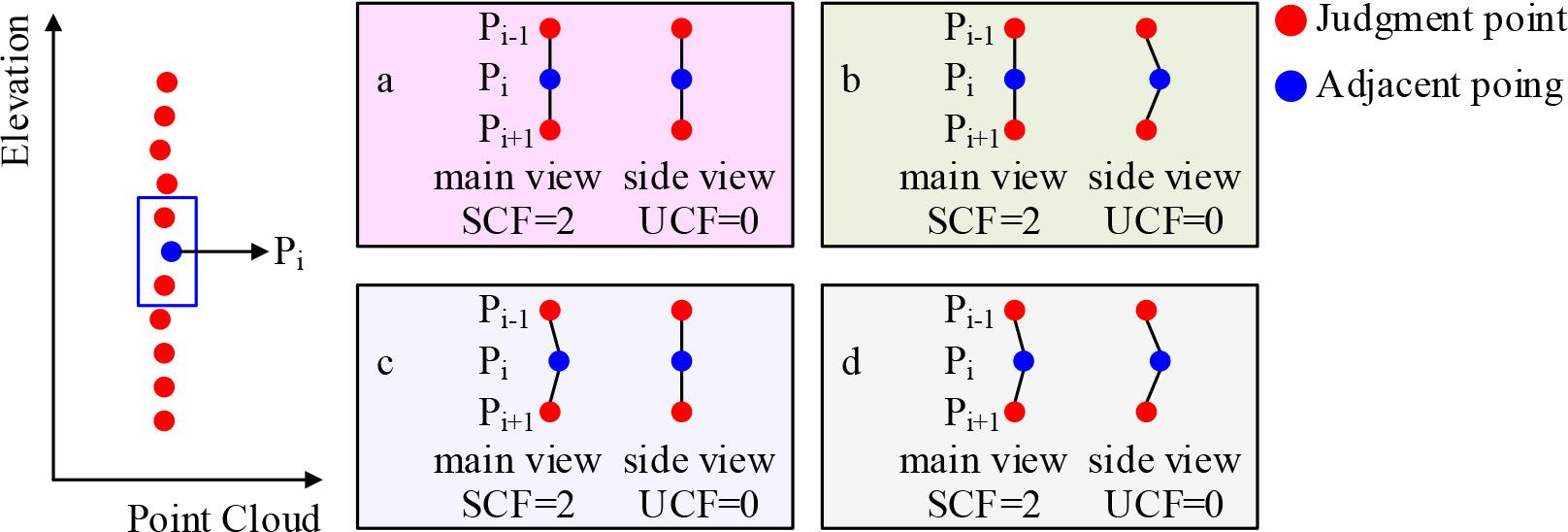
Initial window determination, firstly construct the initial window, determine the number of window point sets as 3, and join the starting position of scanning line No.1 to be a thinned point cloud with two proximity points.

2)

Calculate the angle, and then calculate the value of the angle formed by the thinning points and the proximity points in the window according to the formula (26) θ . (26) $θ = \arccos \frac{\vec{a} * \vec{b}}{| \vec{a} | * | \vec{b} |}$ Where: $\vec{a}$ , $\vec{b}$ are the composition vectors of the cloud of points to be thinned and the two proximity points, respectively.

3)

Calculate the eigenvalues, according to formula (27), to calculate the concave-convex characteristic similarity value (SCF) and the number of outliers (UCF) of the thinning point and other points, the initial value of the number of 0, in order to ensure the accuracy of the detection, the control error within ±1mm, according to the formula (25) to find out the range of the angle of conditions for ±6.12″. When the conditions are met, θ = 180°±6.12°, SCF value increases by 1, when the conditions are met, θ ≠ 180°±6.12° , the value of the UCF increases by 1: (27) ${\begin{array}{l} S C F = S C F + 1 (θ = 180 ° \pm 6.12 °) \\ U C F = U C F + 1 (θ \neq 180 ° \pm 6.12 °) \end{array}$

Figure 1 shows the principle of concave-convex feature point judgement, point P_i is to be thinning point, according to the formula (26) to calculate P_i and its proximity to the two points P_i−1, P_i+1 of the angle value, according to the formula (27) to calculate the SCF and UCF, Figure 1 in the window point set of concave-convex distribution of the four cases, the four cases, a for the smooth distribution of the dilution can be given to the retention of concave-convex features, b, c, d are present.

4)

Sliding window, traversing all the scanned data, according to the above feature point judgement criteria, to complete the scanning data points non-uniform thinning.

Effective extraction of point cloud data features and plane fitting is a prerequisite for the application of 3D laser scanning technology in inspection work. This paper uses the RANSAC algorithm combined with the eigenvalue method for automated feature extraction and plane fitting of 3D point cloud data to obtain accurate plane fitting parameters, and then realizes the detection of multi-indicators. The algorithm process is as follows:

3.2

Detection Principles

3.2.1

Plane extraction and fitting based on the RANSAC eigenvalue method

Effective extraction of point cloud data features and plane fitting is a prerequisite for the application of 3D laser scanning technology in inspection work. This paper uses the RANSAC algorithm combined with the eigenvalue method for automated feature extraction and plane fitting of 3D point cloud data to obtain accurate plane fitting parameters and then realise the detection of multi-indicators. The algorithm process is as follows: 1)

First, three points are randomly selected from all known 3D point cloud data, and then judge whether these three points are co-linear or not. If they are co-linear, then they have to be randomly selected again, and if they are not co-linear, then calculate the plane equations corresponding to these three points according to equation (28): (28) $A x + B y + C z + D = 0$ Where: A, B, C, D are parameters of the plane equation.

2)

Calculate the distance of each point in the point cloud to the above plane based on equation (29) d_i: (29) $d_{i} = \frac{| A x_{i} + B y_{i} + C z_{i} + D |}{\sqrt{A^{2} + B^{2} + C^{2}}}$

3)

Calculate the standard deviation σ of the distance d_i from each point to the plane based on equation (30): (30) $σ = \sqrt{\frac{\sum_{i = 1}^{n} {(d_{i} - \bar{d})}^{2}}{n - 1}}$ Where: $\bar{d} = \frac{1}{n} \sum_{i = 1}^{n} d_{i}$ . t = 2σt = 3σd_i>t.

The standard deviation is a measure of the extent to which the data values deviate from the arithmetic mean, and the standard deviation of the distance from the point to the model plane is used as a criterion for judging the internal and external points. Normally, a threshold value of t = 2σ is taken, but considering that the topological spatial relationship from the point to the fitted plane is also used in the construction building flatness inspection work, in order to avoid the loss of wall inspection features due to the plane extraction, an intermediate value of t = 3σ is taken. When d_i>t is taken, the point is considered to be an out-of-boundary point, and it is deleted. On the contrary, it is considered as an in-local point and the point is retained.

4)

Repeat steps 1)-3) for M iterations, and set the number of threshold points according to the scanning point interval and the size of the detected wall surface, e.g., the scanning point interval is 1cm, the length and width of the detected wall surface are 4m and 3m, respectively, and the number of threshold points is 120701. Compare and select the model with the highest number of points in the bureau to get the set of points to be fitted, a total of n data points. The robust eigenvalue method was used for plane fitting, which satisfies Eq. (31) under condition A² + B² + C² = 1: (31) $e = \sum_{i = 1}^{n} d_{i}^{2} = \sum_{i} {(A x_{i} + B y_{i} + C z_{i} - D)}^{2} \to \min$

5)

Use the Lagrange multiplier method for finding the extreme values of a function to form the functional equation (32): (32) $f = \sum_{i} d_{i}^{2} - λ (A^{2} + B^{2} + C^{2} - 1)$

6)

Derive Eq. (28) for A, B and C respectively and make the derivative zero, then construct the eigenvalue equation and solve the eigenvectors corresponding to the smallest eigenvalues as the fitting parameters A, B and C.

7)

Repeat steps 1)-6) for the remaining set of out-of-bounds points to obtain the fitted parameters for each plane of the building.

3.2.2

Dimensional inspection

1)

Obtain the floor, wall and floor fitting equations: A_iX+B_iY+C_iZ+D_i = 0 , A_i, B_i, C_i, D_i are the plane equation parameters.

2)

Associate the floor and wall equations, floor and wall equations, respectively, to obtain two intersection line equations. Then the normal vector of the intersection line is: (33) $\vec{s} = (m, n, q) = (\begin{matrix} \vec{i} & \vec{j} & \vec{k} \\ A_{1} & B_{1} & C_{1} \\ A_{2} & B_{2} & C_{2} \end{matrix})$

3)

According to the requirements of the specification for axial dimension testing, the intersection line is divided into three equal parts, each of which is set up as a separate segment. Take a point in each equal segment, counted as point: p_i = (x_i,y_i,z_i). If in the two lines of intersection in each equal segment respectively take point: p₁ = (x₁,y₁,z₁) p₂ = (x₂,y₂,z₂), then $\vec{v} = (x_{2} - x_{1}, y_{2} - y_{1}, z_{2} - z_{1})$

4)

The height of storey $\bar{d}$ is: (34) $d_{i} = \frac{| \vec{s} \times \vec{v} |}{| \vec{s} |}$ (35) $\bar{d} = \frac{1}{n} \sum_{i = 1}^{n} d_{i}$

3.2.3

Levelling tests

1)

Use the robust eigenvalue method to obtain the equation of the plane to be inspected as: Ax+By+Cz+D = 0, A, B, C and D are the parameters of the plane equation.

2)

Set the coordinates of the points in the plane as: (m_i,p_i,q_i). Calculate the orthogonal distance and the centre error from each point of the wall to be inspected to the fitted plane according to Eqs. (36) and (37), respectively: (36) $d_{i} = \frac{| m_{i} A + p_{i} B + q_{i} C + D |}{\sqrt{A^{2} + B^{2} + C^{2}}}$ (37) $\bar{d} = \frac{1}{n} \sum_{i = 1}^{n} d_{i}$

3)

Calculate the flatness of the wall to be tested according to formula (38): (38) $s = \sqrt{\frac{\sum_{i = 1}^{n} {(d_{i} - \bar{d})}^{2}}{n - 1}}$ where s is the flatness.

3.2.4

Verticality check

1)

The equations of the wall to be inspected are obtained using the medium fitting method as: A₁X+B_iY+C_iZ+D_i = 0, A_i, B_i, C_i and D_i are the parameters of the plane equations.

2)

Select the reference plane. In the construction of the building project certain floor slabs are set up with a certain slope, so the fitted floor surface is not suitable as the reference plane. Therefore, XY planes in the vertical direction are selected as the reference plane and the plane equations are derived: (39) $A_{k} x + B_{k} y + C_{k} z + D_{k} = 0$

In the formula, A_j, B_j, D_j = 0, C_j = 1.

3)

Calculate the angle between the wall to be tested and the reference plane: (40) $α = \arccos \frac{| A_{i} A_{k} + B_{i} B_{k} + C_{i} C_{k} |}{\sqrt{A_{i}^{2} + B_{i}^{2} + C_{i}^{2}} \sqrt{A_{k}^{2} + B_{k}^{2} + C_{k}^{2}}}$ Where α is the angle between the wall to be detected and the reference plane.

4)

Calculate the verticality of the plane to be tested: (41) $v = \tan θ = \tan (90 - α), v = {\begin{array}{l} v, α \leq 90 ° \\ | v |, α > 90 ° \end{array}$

4

Empirical analyses of structural safety inspections of urban dwellings

4.1

Structural safety inspection of housing based on streak array detection

4.1.1

Accuracy assessment

The three-dimensional model of urban housing structure is decomposed into primitive lines and primitive points using streak array detection, and then the overall accuracy of the three-dimensional model of urban housing is analysed according to the evaluation of local accuracy. Firstly, the 3D model of urban housing is imported into EPS analysis software, and 20 building point coordinates and 10 side lengths are selected. Secondly, the field measurement of urban housing buildings is carried out manually by using a rangefinder and total station, and the actual parameters of building coordinates and side lengths of the measurement points are counted, and the statistical results are shown in Table 1.

Table 1.

Statistical result

Precision index		Δx	Δy	Δz	Δs	Δl
Model measurement	Measurement point 1	29.458	30.548	66.158	9.085	11.758
	Measurement point 2	28.456	33.415	71.585	12.267	12.248
	Measurement point 3	34.598	31.578	69.288	13.485	14.925
External measurement	Measurement point 1	30.278	30.524	70.488	9.158	9.514
	Measurement point 2	29.578	30.248	67.285	8.328	13.537
	Measurement point 3	29.178	30.297	68.274	10.595	11.918
Maximum error		4.258	-3.275	3.718	4.812	5.418
Minimum error		-0.485	0.378	-0.548	0.785	2.258
Middle error		2.587	2.185	1.617	3.158	3.245

As can be seen from Table 1, the minimum measurement error between the urban housing 3D model measurement points and the field measurement points in the direction of the X-axis is -0.485cm, the maximum measurement error is 4.258cm, and the median error is 2.587cm. In the direction of the Z-axis and Y-axis, the minimum measurement error is -0.548cm, 0.378cm, and the maximum measurement error is 3.718cm, -3.275cm, and the median error is 3.718cm, -3.275cm. 3.275cm, and the median error is 1.617cm, 2.185cm. The UAV from the measurement points Δs and Δl, the minimum measurement error is 0.785cm, 2.258cm, the maximum measurement error is 4.812cm, 5.418cm, and the median error is 3.158cm, 3.245cm.

4.1.2

Verification of structural system and overall soundness

After on-site inspection, the total length of the building is about 35.8m, the total width is about 9.2m, rectangular distribution, the height of the ground floor and the second floor are 3.6m, the room openings are 3.9m and 4.0m, the depths are 7.2m and 9.2m, respectively. The corridor is set up on the south side, and the corridor is 2.0m in width. The load-bearing walls are made of sintered clay and mixed slurry masonry, of which the thicknesses of the two ends of the mountain wall, the A-axis and the C-bearing walls are 370mm, and the thicknesses of the rest of the vertical and horizontal walls are 240mm. The thickness of the two end walls, A-axis and C-bearing walls, is 370mm, while the thickness of the remaining load-bearing walls is 240mm. There is no ring beam at the top of each floor, and there are structural columns in the 3/B-axis, 5/B-axis and 8/B-axis, and there are no structural columns in the remaining longitudinal and transversal wall junctions and corners, and the floor panels and the roof panels are cast-in-situ reinforced concrete slabs.

The results of the structural testing of housing are displayed in Table 2. The conversion value of compressive strength of masonry mortar of sampled walls is 3.948~4.525MPa, the conversion value of compressive strength of masonry bricks of sampled walls is 7.376~8.257MPa, and the presumed strength of concrete of sampled beams of current age is 23.551~26.487MPa, and the depth of carbonation of some measurement points has exceeded the thickness of protective layer of steel reinforcement required by the specification. On-site sampling of the top 3/B~C axis beam of the first floor, chiseling the bottom corner of the beam part of the concrete, the measured corner of the main reinforcement for a diameter of 20mm rebar, and hoop diameter of 8mm round steel. The spacing of reinforcing bars at the bottom of the sampled cast-in-situ slab was 132~242mm. The wall cracks on the ground floor of the house were more, and after analysis, the wall cracks of the house were mainly caused by the uneven settlement of the foundation, and the building was not found to be affected by the lack of bearing capacity on the superstructure.

Table 2.

Housing structure test results

Member		Conversion value of masonry mortar resistance(MPa)		Conversion value of brick resistance(MPa)
Name	Axis number	Conversion value of masonry mortar resistance(MPa)		Conversion value of brick resistance(MPa)
Ground wall	6~7/B	3.948		8.257
Ground wall	4/B~C	4.325		7.376
Two-story wall	1~2/A	4.525		7.829
	3~4/B	3.974		8.156
	7~8/B	4.525		7.596
Member		Concrete anti-pressure conversion value(MPa)			The value of the strength of the cloud coagulation soil in the present age(MPa)
Name	Axis number	Mean value	Standard deviation	Minimum value
Top beam	8/B~C	28.287	2.375	24.915	24.596
Top beam	6/A~B	28.653	1.818	25.631	25.485
Second floor top beam	3/B~C	29.185	2.569	26.278	25.385
	3/A~B	29.675	1.975	27.168	26.487
	8/B~C	29.169	3.278	27.294	23.551
Test floor	Axis number	Measured beam base number		The measured band is the average spacing(mm)	The measured cross section width×height(mm)
A top beam	8/B~C	4 root		Full section:205	254×505
	6/A~B	5 root		Full section:215	253×207
	5~6/B	4 root		Full section:208	257×204
Two-story roof beam	3/B~C	3 root		Full section:204	257×536
Two-story roof beam	3/A~B	2 root		Full section:210	254×206
Member		Average spacing of bar
Name	Axis number	Steel direction	Measured measurement (mm)	Steel direction	Measured measurement(mm)
Top plate	7~8/B~C	7↔9	132	B↔C	187
Top plate	6~7/A~B	5↔6	242	A↔B	235
Two deck roof	9~10/A~C	8↔10	149	A↔C	157
Two deck roof	3~4/B~C	4↔5	164	B↔C	198

4.2

Detection results and prediction of detection results

4.2.1

Inspection of building structural data

Because of the large number of buildings and monitoring contents monitored in this project and a large amount of data, the monitoring data of the rear building of No. 37 at a certain location at a certain time period from 15 May 2023 to 19 May 2023 are analysed in this paper. The settlement monitoring, tilt monitoring, and horizontal displacement at a point of the tested housing are shown in Table 3. In the settlement detection data, the settlement change on the day of 2023.5.15 was the highest among the five days, and in the tilt detection data, the tilt data in the z-axis remained in the range of 88.49 to 88.97. The longest two-dimensional displacement length data occurred at 16:00 hrs on 2023.5.16, which was 5.454.

Table 3.

Test data

	Sedimentation detection data(mm)
	2023.5.15		2023.5.16		2023.5.17		2023.5.18		2023.5.19
	8:00	16:00	8:00	16:00	8:00	16:00	8:00	16:00	8:00	16:00
Varying quantity	4.846	3.685	4.158	3.512	4.186	3.285	4.082	3.188	4.285	3.282
Varying quantity	Tilt detection data(°)
	2023.5.15		2023.5.16		2023.5.17		2023.5.18		2023.5.19
	8:00	16:00	8:00	16:00	8:00	16:00	8:00	16:00	8:00	16:00
X	-1.285	-1.562	-1.065	-1.156	-1.089	-1.087	-1.048	-1.096	-1.152	-1.065
Y	-0.789	-0.758	-0.768	-0.685	-0.728	-0.625	-0.526	-0.725	-0.755	-0.526
Z	88.485	88.685	88.957	88.964	88.765	88.756	88.966	88.755	88.645	88.845
Varying quantity	Horizontal displacement detection data(mm)
	2023.5.15		2023.5.16		2023.5.17		2023.5.18		2023.5.19
	8:00	16:00	8:00	16:00	8:00	16:00	8:00	16:00	8:00	16:00
X	1.758	2.162	2.218	3.948	3.942	1.925	1.826	1.822	1.826	1.526
Y	-3.865	-4.263	-4.531	-3.156	-3.815	-4.328	-3.255	-4.458	-3.157	-3.128
Two dimensional displacement length	4.125	4.684	5.035	5.454	3.655	4.728	4.062	5.063	3.566	4.053

4.2.2

Structural materials

The rebound test is carried out on building concrete members using testing tools, thus reflecting the strength index of concrete structural members. In this sampling, all vertical members were taken for testing, and 20 per cent of all horizontal floor members were taken for testing. Therefore, this strength testing work can fully reflect the current status of the concrete strength of the building housing. Based on the actual test data obtained, the strength of the reinforced concrete members of the residential building is inferred. The strength test of concrete in urban housing is displayed in Table 4. From the table, it can be seen that after 3D mapping, it can be seen that in the concrete structure of the housing, the highest mean value of rebound of 1.235 was found in the floor slabs and walls on the second basement level. The lowest value of rebound was found in the floor slabs and walls on the ground floor level, which was only 0.9365.

Table 4.

Measurement of concrete strength of urban housing

Floor	Build Type	Constructive strength(Mpa)	Design strength(Mpa)	Rebound value/design value
Sublayer	Floor Slab	30.345	30	1.185
Sublayer	Wall	36.585	30	1.285
Underground Layer	Floor Slab	32.748	30	1.093
Underground Layer	Wall	38.128	30	1.275
Layer	Floor Slab	24.374	27	0.925
Layer	Wall	28.945	30	0.948
Second Layer	Floor Slab	24.348	26	0.972
Second Layer	Wall	29.348	25	0.974
Three-Ply	Floor Slab	27.845	25	1.156
Three-Ply	Wall	28.148	24	1.136
Four-Ply	Floor Slab	24.263	26	0.948
Four-Ply	Wall	24.317	25	0.978
Pentinterval	Floor Slab	28.183	25	1.132
Pentinterval	Wall	24.425	26	0.925
Sexosphere	Floor Slab	24.382	25	0.985
Sexosphere	Wall	24.874	26	0.974
Heptad	Floor Slab	25.365	25	1.088
Heptad	Wall	29.348	25	1.148
Octal Layer	Floor Slab	25.558	25	1.054
Octal Layer	Wall	28.533	26	1.154
Nine Floors	Floor Slab	24.728	25	0.948
Nine Floors	Wall	28.348	25	1.184
Decida	Floor Slab	24.918	26	0.978
Decida	Wall	28.365	25	1.126
Ten Layers	Floor Slab	30.482	25	1.254
Ten Layers	Wall	28.485	26	1.156

4.3

Finite element analysis of settlement management

4.3.1

Finite Element Analysis of Uneven Settlement of Superstructure Rigidity

Uneven settlement of the foundation will affect the superstructure, especially the ground floor. When the relative settlement difference is too large, it will also cause the additional axial force, additional bending moment, and additional shear force of beams and columns on the ground floor to exceed the normal service limit of the member. In contrast, the impact on the first floor and above it is relatively small, and the difference is not significant.At the same time, the impact on the ground floor is the most significant after the addition of the study object, and the impact on the first floor and above it is relatively small.

According to the degree of impact, the structural reinforcement of the most affected ground floor is the primary reinforcement target in the management of uneven settlement of houses. But at the same time, affected by the smaller first floor and the first floor above the structural components need to be reinforced? What is the effect of reinforcement on the overall stability of the house? Forces act on each other, since the uneven settlement of the foundation will have an impact on the superstructure, then the change of the superstructure will inevitably also have an impact on the settlement of the foundation. This chapter is a reverse analysis of the change of the first floor and the first floor above the structural rigidity to analyse the effect of uneven settlement, through the effect of uneven settlement effect of the weakening role, so as to reflect the overall stability of the house from the side of the role of the size.

4.3.2

Finite element modelling

In the finite element modeling analysis, the stiffness of the upper beams and columns is gradually changed in layers to analyze the change in the amount of inhomogeneous settlement under various scenarios. The steps are as follows: 1)

The initial concrete strength of the structure is all taken as C20, the density of reinforced concrete is uniformly 2400kg/m³, the elastic modulus of C20 concrete is taken as 2.55*104MPa, of which the elastic modulus of columns is initially 2.55*104MP, and then it is upgraded step by step according to the “Code for the Design of Concrete Structures” GB50010-2002.

2)

Gradually change the elastic modulus of the columns in the second level, and analyse the additional settlement on the settling columns as well as the surrounding columns.

3)

Following the same steps, the elastic modulus of the columns in the third, fourth, and fifth layers were individually changed, calculated and analysed.

4.3.3

Analysis of finite element calculation results

Table 5 displays the additional settlement values for each settling column after the modulus has been modified. By modifying the elastic modulus of the second layer, the second layer perimeter, the third layer, and the fourth layer columns individually, it was found that all of them had a certain amount of settlement weakening effect on the bottom layer columns. In terms of the effect, when the modulus of elasticity was modified from 2.55*10⁴MPa to 2.80*10⁴MPa, it had a positive effect on the settlement of both the bottom settled columns and the peripheral columns, and it was learnt from the analysis of the additional settlement values of the second layer of the settled columns that the settlement values of each of the columns were 24.588, 27.841, 28.854, 32.182, 33.148, and 27.398, respectively, 31.985 and the settlement value is ranked first. However, when the modulus of elasticity was gradually revised to 3.0*10⁴MPa, 3.15*10⁴MPa, 3.25*10⁴MPa, the effect was basically unchanged, and when the modulus of elasticity was modified in the second, third and fourth layers, the difference in the effect played in the three cases was very small. It can be seen that in the uneven settlement of the house, through the reinforcement of the second layer and, the second layer above can play a certain range of roles has a certain upper limit, which corresponds to the uneven settlement of the foundation on the second layer and the second layer above the impact of the small and not much difference.

Table 5.

Additional sedimentation of each sedimentation column after modification of modulus

^E*10⁴MPA	Column 1-A	Column 1-D	Column 5-A	Column 5-D	Column 9-A	Column 14-A	Column 14-D
2.8	24.588	27.841	28.854	32.182	33.148	27.398	31.985
3	24.515	27.534	28.015	32.175	33.145	27.215	31.948
3.15	24.562	27.523	28.063	32.139	33.125	27.305	31.974
3.25	24.589	27.585	28.089	32.135	33.147	27.396	31.915
^E*10⁴MPA	Column 2-A	Column 2-B	Column 2-C	Column 2-D	Column 3-A	Column 3-B	Column 3-C
2.8	25.052	26.875	27.245	27.859	25.688	26.895	27.918
3	25.036	26.615	27.268	27.915	25.684	26.947	27.936
3.15	25.048	26.588	27.687	27.951	25.688	26.974	27.927
3.25	25.054	26.856	27.456	27.956	25.614	26.974	27.936
^E*10⁴MPA	Column 1-A	Column 1-D	Column 5-A	Column 5-D	Column 9-A	Column 14-A	Column 14-D
2.8	24.598	27.458	28.096	32.148	33.168	27.896	31.785
3	24.566	27.966	28.156	32.138	33.184	27.596	31.998
3.15	24.515	27.628	28.104	32.185	33.125	27.398	31.248
3.25	24.578	27.885	28.196	32.145	33.169	27.398	31.958
^E*10⁴MPA	Column 1-A	Column 1-D	Column 5-A	Column 5-D	Column 9-A	Column 14-A	Column 14-D
2.8	24.597	27.612	28.485	32.175	33.184	27.652	32.087
3	24.605	27.614	28.996	32.148	33.148	27.518	32.007
3.15	24.633	27.628	28.154	32.336	33.195	27.369	32.065
3.25	24.604	27.988	28.745	32.174	33.178	27.965	32.014

By modifying the analysis of the elastic modulus of the superstructure of the house, it is learnt that the result of reinforcing the first floor and above can play a certain role in the stability of the house, but the effect is limited. Therefore, when strengthening the house, we mainly start from the bottom layer, which is most affected by the settlement, and according to the actual situation, we can assist in the reinforcement of the second layer and above.

5

Conclusion

In this paper, a striped array detection lidar is constructed, and the target distance is determined with high accuracy using the centre-of-mass weighting method.The inertial navigation system and the distance inversion method are respectively used to obtain distance image coordinate information in the geodetic latitude and longitude coordinate system. The RANSAC algorithm combined with the eigenvalue method is used to extract the 3D cloud data features, and empirical analyses are carried out to detect the safe structure of urban housing from three perspectives: size, flatness, and verticality.

In the data accuracy assessment of urban housing structures, the minimum measurement error in the X-axis direction is -0.485cm, while the maximum measurement error is 4.258cm, and the median error is 2.587cm. In the Z-axis and Y-axis direction, the minimum measurement error is -0.548cm, 0.378cm, and the maximum measurement error is 3.718cm, -3.275cm, and the median error is 1.617cm, 2.185cm. cm, 2.185 cm. The errors are within reasonable limits.

The system and overall solidity of the housing structure were tested, and the converted values of compressive strength of masonry mortar of sampled walls, converted values of compressive strength of masonry bricks of walls, and presumed values of concrete strength of beams at the present age were 3.948~4.525MPa, 7.376~8.257MPa, and 23.551~26.487MPa, respectively, and the cracks of the walls of the houses were mainly due to the uneven settlement of the foundations. The uneven settlement of the foundation mainly caused cracks in the walls of the houses, and there was no influence on the superstructure due to the insufficient bearing capacity of the building.

The stiffness of the upper beams and columns gradually changed in layers, and the degree of change in their uniform settlement in different cases was analysed by finite element modelling. When the modulus of elasticity was modified from 2.55*10⁴MPa to 2.80*10⁴MPa, it had a positive effect on the settlement of the bottom settled columns and the peripheral columns, and the settlement values of the columns in the second layer were 24.588, 27.841, 28.854, 32.182, 33.148, 27.398, and 31.985, and the settlement values were enhanced significantly.

Funding:

This research was supported by the Research Project of Henan Federation of Social Science: Construction and Research of Ideological and Political Teaching in College Curriculum - Taking Civil Engineering Survey as an Example (Project Number: Skl-2022-778).

Language:: English

Publication timeframe:: 1 times per year
Journal Subjects:: Life Sciences, Life Sciences, other, Mathematics, Applied Mathematics, General Mathematics, Physics, Physics, other

Journal RSS Feed

Application of high-precision three-dimensional mapping technology in urban housing structural safety inspection

Peijie Yu

Yanlun Liu

Published Online: Mar 17, 2025

Received: Oct 09, 2024

Accepted: Feb 04, 2025

DOI: https://doi.org/10.2478/amns-2025-0174

KeywordsStriped column detection, Centre of mass weight method, RANSAC algorithm, Structural safety detection

© 2025 Peijie Yu et al., published by Sciendo

This work is licensed under the Creative Commons Attribution 4.0 International License.

Keywords
Striped column detection, Centre of mass weight method, RANSAC algorithm, Structural safety detection