Load Distribution Prediction and Design Models for Ship Special Mechanical Devices and Equipment under Non-linear Sea Conditions

Published Online: Mar 17, 2025
Received: Nov 09, 2024
Accepted: Feb 09, 2025
DOI: https://doi.org/10.2478/amns-2025-0170
Keywords
© 2025 Peiyao Yang, published by Sciendo
This work is licensed under the Creative Commons Attribution 4.0 International License.
Ships are generally composed of hull structure, power plant, power plant systems, piping systems, and oil and water tanks and equipment compartments, etc., with a solid structural composition, good sea performance and loading and transportation capacity; these functions require some high parameters of the load-bearing equipment, high-specification electromechanical equipment, such as “special equipment” to support the protection [1-3]. Ship special equipment used in harsh environments, complex operating conditions, and the risk of hidden danger, once the problem directly affects the ship’s life safety, is major high-risk equipment [4-6]. With the continuous expansion of the cruise range of the ship, the possibility of encountering adverse sea conditions has greatly increased. When the ship with a large external drift speed in bad sea conditions, easy to be affected by the violent impact of the bang load and the hull movement will produce significant nonlinear phenomenon, high sea state of the hull of a large movement in the nonlinear phenomenon is more obvious [7-10]. A large number of experiments have proved that the time-record results of hull motion and wave loading in severe sea states have obvious nonlinearities [11-12]. The large motion of the ship in a nonlinear sea state will generate a large inertia load, and the waves surging on the deck will also have an impact on the ship equipment, threatening the safety of the ship equipment [13-15]. Therefore, how accurately predict the motion loads of ships under severe sea state provides a certain reference value for ship navigation and the safety guarantee of special mechanical devices and equipment.
In order to improve the accuracy of forecasting large ship motions, nonlinear factors in the motions need to be taken into account. Literature [16] shows that the structural rules of a ship specify various loads corresponding to the ship in the most severe sea state to provide safety, but most of its assessments are based on linear wave resistance coding and linear statistical prediction preparation formulas, which are unable to adapt to the complex sea state, so fiber grating sensors are introduced to measure in detail the numerical calculations of different ships in both regular and irregular waves, which are used to assess the structural strength of the ship. Literature [17] discusses the advantages and disadvantages of numerical prediction methods in the structural assessment of ships subjected to steady state or transient excitation loads and also evaluates the uncertainty in predicting wave-induced loads, as well as probabilistic methods for evaluating the long-term response and fatigue analyses to lay the foundation for the development of wave load prediction for ships. Literature [18] proposes a large-scale model measurement technique with better applicability and versatility to predict the short-term motion and load response of a ship under the corresponding sea state by measuring its wave resistance and wave load characteristics in different hydrodynamics, in addition to the long-term extreme prediction of the motion load based on the numerical results of the short-term prediction. Literature [19] designs a relatively simplified nonlinear method to predict the pendulum motion, pitching motion and vertical bending moment of a container ship on the basis of the three-dimensional time-domain panel method, including an algorithm for accurately solving the dipping surface under the incident wave profile and an estimation method for the correction of the object’s motion conditions, and the experiments show that the proposed method can efficiently estimate the wave-induced nonlinear response.
Some scholars have predicted the equipment loads under nonlinear sea state to assess the safety risk of marine special equipment use. Literature [20] used a three-dimensional, fully nonlinear time domain model based on the boundary element method to analyze the nonlinear dynamic response of the suspended loads of lifting vessels, to study the dynamic characteristics of the underwater loads of offshore lifting vessels, and to use this as a basis for designing techniques to control or damp the unexpected motion of underwater loads. Literature [21] studied the dynamics and robust control problems of the wave compensation system of marine robotic arms under complex sea conditions, introduced nonlinear differential and integral sliding mode control strategies to improve the stability of the dynamic control system of marine robotic arms, and also provided useful references for the wave compensation systems of other marine equipment. Literature [22] establishes an electromechanical-hydraulic coupling dynamics model of the shipboard gun that includes the influence of the follower system and adopts a bilaterally symmetric tooth arc arrangement scheme to reduce the influence of the ship’s base motion excitation on the accuracy of the shipboard gun, which provides theoretical support for the relevant design of the shipboard gun.
In this paper, the second-order Stokes wave and Ochi-Hubble six-parameter bimodal wave spectrum are combined to achieve the environmental modelling of nonlinear mixed sea state, and then numerical simulation is carried out based on the fluid-structure coupling method combining the Computational Fluid Dynamics (CFD) and the Finite Element Method (FEM) to complete the prediction of load distribution of the ship’s special mechanical devices and equipments under the nonlinear sea state. Taking the pump-jet thruster as an example, the optimal design of load distribution is carried out according to the prediction results, and it is verified whether the designed load distribution meets the requirements.
Ship special machinery refers to the special mechanical devices that can meet the needs of a ship’s special performance, including the rocking device, pitch paddle device, ship lift, and special conveyor devices. With the ship’s comfort, safety, economy, and other requirements, the focus has gradually shifted to equipping civilian ships.
Under severe sea conditions, the environmental loads such as wave force, wind force and current force to which the ship is subjected when sailing at high speed have significant uncertainty, coupling and time-varying nature, which makes the ship motion process show obvious nonlinear characteristics.
Therefore, non-linear sea state usually refers to irregular variations and interactions of natural factors such as waves, currents, winds, etc., which may lead to a significant increase in the six-degree-of-freedom motions of the ship (longitudinal swing, transverse swing, plumb swing, transverse rocking, longitudinal rocking, and bow rocking), which may result in complex dynamic loads on specialised mechanical installations and equipments on board the ship.
The load distribution in a nonlinear sea state is mainly characterized by the following characteristics:
Dynamic variability In a non-linear sea state, the wave force and wind force to which the ship is subjected are often irregular and changing, which leads to a non-linear motion response of the ship. Therefore, the special mechanical devices and equipment on the ship must be able to adapt to dynamically changing load conditions to ensure normal operation under various circumstances. Uneven structural stress The complex motion environment in a non-linear sea state will lead to uneven stress distribution in the ship structure. This requires shipping special mechanical devices and equipments to take into account the maximum stresses on different parts during design and how to disperse these stresses through reasonable structural design and material selection to avoid structural damage or fatigue damage. Vibration and shock absorption requirements The violent movement of the ship under severe sea conditions will generate large vibrations and impacts, which is a severe test for the shipboard equipment. Therefore, these energies need to be absorbed by installing shock absorbers and vibration isolation systems to protect sensitive equipment from damage. Energy management optimisation Under a non-linear sea state, the energy consumption pattern of the ship will change, especially in the propulsion and stabilization systems. Therefore, an intelligent energy management system is needed to optimize the distribution and usage efficiency of energy to ensure the safety of the ship’s energy supply during a long voyage. Control system adaptability In order to address the challenges posed by non-linear sea conditions, the ship’s control system must be highly adaptable and flexible. This means that the control system needs to be able to detect environmental changes in real-time and quickly adjust the ship’s speed, heading, and attitude, while ensuring stability and safety.
In order to achieve the prediction of the load distribution of special mechanical devices and equipment of ships under nonlinear sea conditions, this paper introduces the second-order Stokes wave model for nonlinear wave simulation analysis [23]. At the same time, this paper uses the Ochi-Hubble six-parameter wave spectrum, which covers a variety of wave spectral shapes, including surges related to the growth and decay of storms, to simulate the sea state. In order to put the ship’s special mechanical devices and equipment in a nonlinear mixed sea state, the bimodal spectrum of the Ochi-Hubble six-parameter wave spectrum family is chosen in this paper [24].
The free surface wave height
For an irregular sea state characterised by a specific wave spectrum
Where
Where
Shallow-water wave data usually do not follow a linear Gaussian ocean model due to bottom effects. The linear Gaussian ocean model can be corrected by adding a second-order term, and the expression for the second-order term
Where
where
Adding the first-order term and the second-order term, the wave height
The Ochi-Hubble six-parameter wave spectrum can be decomposed into two parts, each containing three parameters in its expression. The total spectrum is obtained by adding the two three-parameter spectra. The expression is given below:Ochi-Hubble:
Where
The six parameters in Eq. 1 can be converted into meaningful wave heights
Values of six parameters
| No. | |||||||
| Most likely | 1 | 0.84Hs | 0.54Hs | 0.70e-0.046Hs | 1.15e-0.039Hs | 3.00 | 1.54e-0.062Hs |
| 95% credibility | 2 | 0.95Hs | 0.31Hs | 0.70e-0.046Hs | 1.50e-0.046Hs | 1.35 | 2.48e-0.102Hs |
| 3 | 0.65Hs | 0.76Hs | 0.61e-0.039Hs | 0.94e-0.036Hs | 4.95 | 2.48e-0.102Hs | |
| 4 | 0.84Hs | 0.54Hs | 0.93e-0.056Hs | 1.50e-0.046Hs | 3.00 | 2.77e-0.112Hs | |
| 5 | 0.84Hs | 0.54Hs | 0.41e-0.016Hs | 0.88e-0.026Hs | 2.55 | 1.82e-0.089Hs | |
| 6 | 0.90Hs | 0.44Hs | 0.81e-0.052Hs | 1.60e-0.033Hs | 1.80 | 2.95e-0.105Hs | |
| 7 | 0.77Hs | 0.64Hs | 0.54e-0.039Hs | 0.61 | 4.50 | 1.95e-0082Hs | |
| 8 | 0.73Hs | 0.68Hs | 0.70e-0.046Hs | 0.99e-0.039Hs | 6.40 | 1.78e-0.069Hs | |
| 9 | 0.92Hs | 0.39Hs | 0.70e-0.046Hs | 1.37e-0.039Hs | 0.70 | 1.78e-0.069Hs | |
| 10 | 0.84Hs | 0.54Hs | 0.74e-0.052Hs | 1.30e-0.039Hs | 2.65 | 2.65e-0.085Hs | |
| 11 | 0.84Hs | 0.54Hs | 0.62e-0.039Hs | 1.03e-0.030Hs | 2.60 | 0.53e-0.069Hs |
The meaningful wave height of the waves in this study,
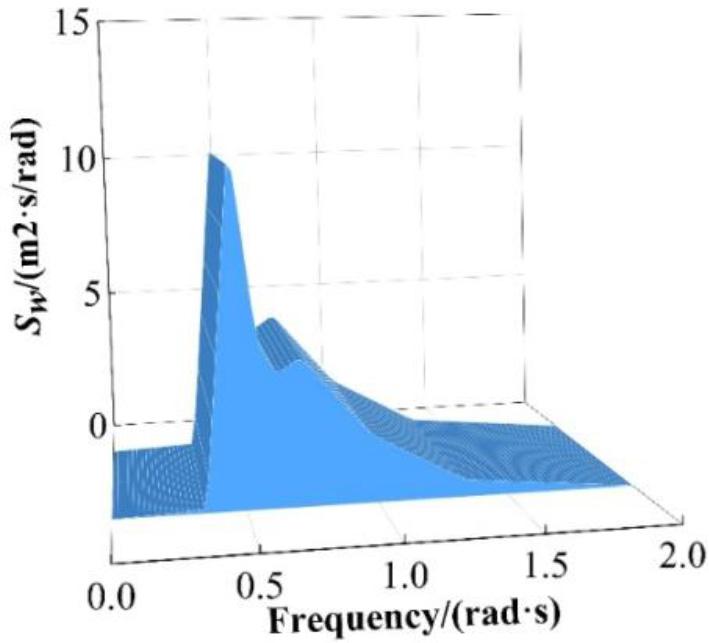
Wave spectrum No. 3
In this paper, a coupled fluid-structure calculation method combining Computational Fluid Dynamics (CFD) and Finite Element Method (FEM) is used, combined with the established nonlinear sea state model, to simulate the loading condition of special mechanical devices and equipment of the ship, so as to achieve the prediction of the load distribution, and to provide a reference for the further optimisation of the design [25].
Fluid control equations
When the compressibility of the fluid is not considered and the surface tension of the fluid is not taken into account, the continuum equation with the N-S equation is used to describe the viscous fluid motion in ocean engineering problems:
Where:
2. Structural control equations
It is assumed that the structure is a linear elastic material, which does rigid body motion and deformation relative to the original equilibrium position under the action of external loads such as waves, and its structural equations of motion are obtained by the finite element method:
Where:
For linear elastic materials, the stress-strain relationship is linear and given by Hooke’s law:
where: is the material tangent coefficient, is the stress, and is the strain.
Turbulence modelling
When solving engineering problems, the continuous equation and the
Where
Numerical wave generation method
Compared to linear waves, non-linear waves have steeper peaks and flatter valleys, presenting an asymmetric curve that is more consistent with actual waves in reality. In this paper, the second-order Stokes wave model and Ochi-Hubble six-parameter wave spectrum are selected for wave simulation.
Numerical wave cancellation method
In order to eliminate the influence of the reflected waves from the object and the reflected waves at the pool exit on the entrance boundary of the velocity wave making, the wave cancellation area will be set up in both the pool entrance area and the exit area as shown in Fig. 2. The numerical pool inlet wave cancellation area is shown in Fig. 2, the forced wave cancellation method is used, and the wave is forced by adding the source term in the momentum equation.
The source term added to the momentum equation in its inlet dissipation region is:
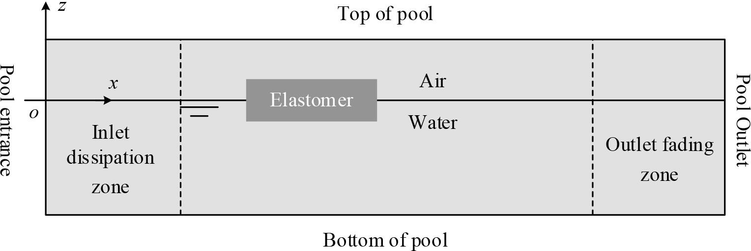
Area of wave damping in numerical tank
Where:
Damping dissipation is used in the numerical pool outlet dissipation zone in Fig. 2 to enhance wave dissipation by adding damping in the vertical direction of wave motion. The additional damping source term in the momentum equation is:
Where:
In the coupling calculation, a two-way coupling method between CFD and FEM is used, and the CFD-FEM two-way coupling process is shown in Fig. 3.
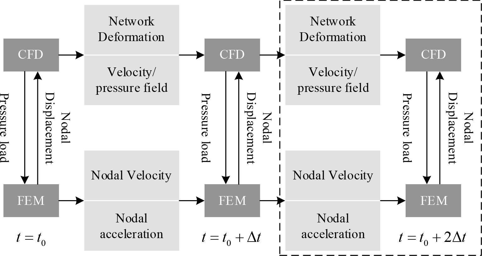
Flowchart of two-way coupling of CFD-FEM
In this paper, the pump jet propeller, a special mechanical device of a ship, is taken as a specific research object, and numerical simulation is carried out by using the CFD-FEM two-way fluid-solid coupling method to predict the load distribution of the ship’s special mechanical device under nonlinear sea state.
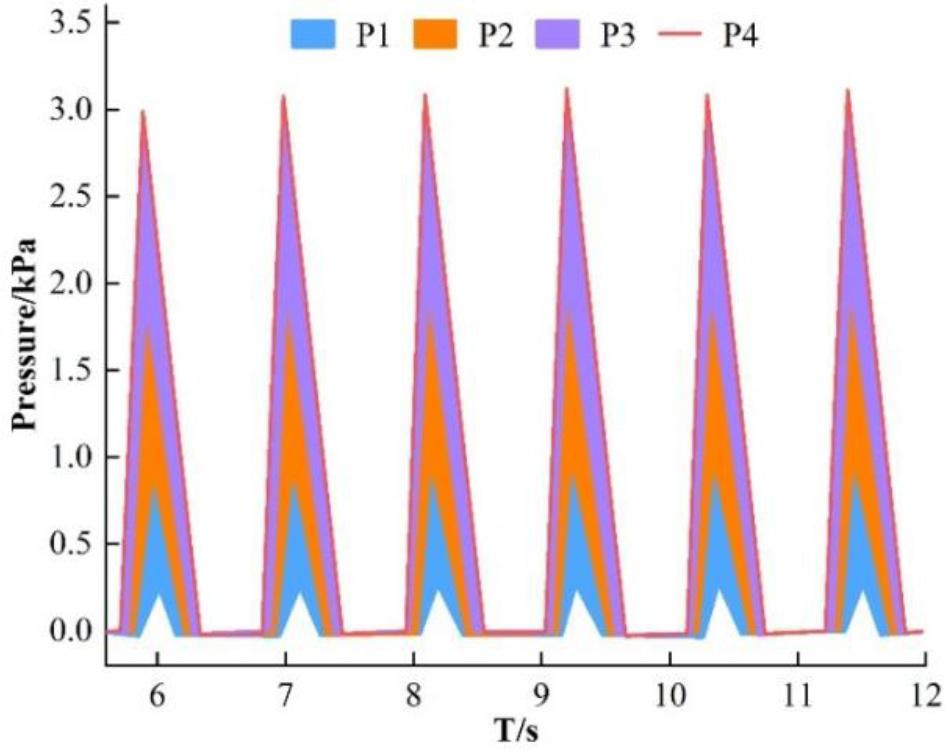
Under the wave condition of wave height H=6m, wavelength to length ratio λ/Lpp=0.87, and sailing with 20kn speed to meet the waves, the CFD-FEM two-way fluid-structure coupling method is used to calculate the load on the pump jet propeller when the hull of the ship and the waves are banging, and the pressure time course of the equidistant measurement points P1~P4 is shown in Fig. 4.
Different measurement points slam the pressure contrast
As can be seen from Fig. 4, the load at measurement point P4 is seriously affected by the thumping action of the ship’s hull, and its peak value exceeds 3.1 kPa. The pressure peaks at measurement points P1 to P4 are more obtuse and decrease with the height of the measurement point, which is due to the fact that the pump-jet propellers are tilted inward, and the angle of their inclination rise is negative.
The loads at measurement point P4 obtained by using the two-way fluid-solid coupling method of test and CFD-FEM are shown in Fig. 5. As can be seen from Fig. 5, the hull thumping cycles of the two ships are consistent, and the amplitude of the load change triggered by the thumping action is similar.
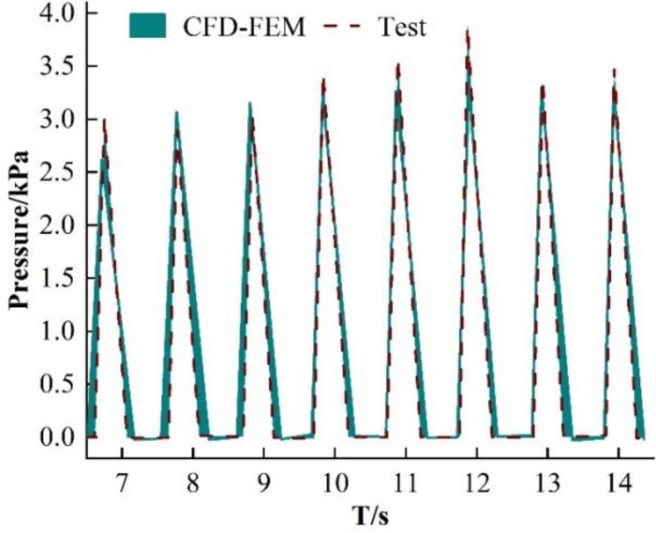
Different measurement points slam the pressure contrast
The load distribution in the pump-jet propeller is mainly expressed as the distribution of blade velocity moment, i.e., the pressure difference between the blade pressure surface and the suction surface.
In this paper, considering the actual sailing conditions of the ship, it is decided to use the intermediate uniform load distribution form that takes into account the efficiency and cavitation of the pump jet thruster, i.e., the load is the largest at 0.2 chord length, and then it is uniformly distributed, and it gradually decreases in the form of 0.6 times the chord length. The blade load distribution of the designed pump jet thruster is shown in Fig. 6. Among them, Figs. (a)~(b) represents the load distribution at the front and rear rotor hubs and rims of the pump jet thruster, respectively, while Fig. (c) represents the guide vane load distribution, given the load distribution at the hubs and rims, and the load distribution at the other radius cross sections is obtained by line interpolation. The load distribution is represented from inside to outside in the figure, and different angles represent multiples of the chord length.
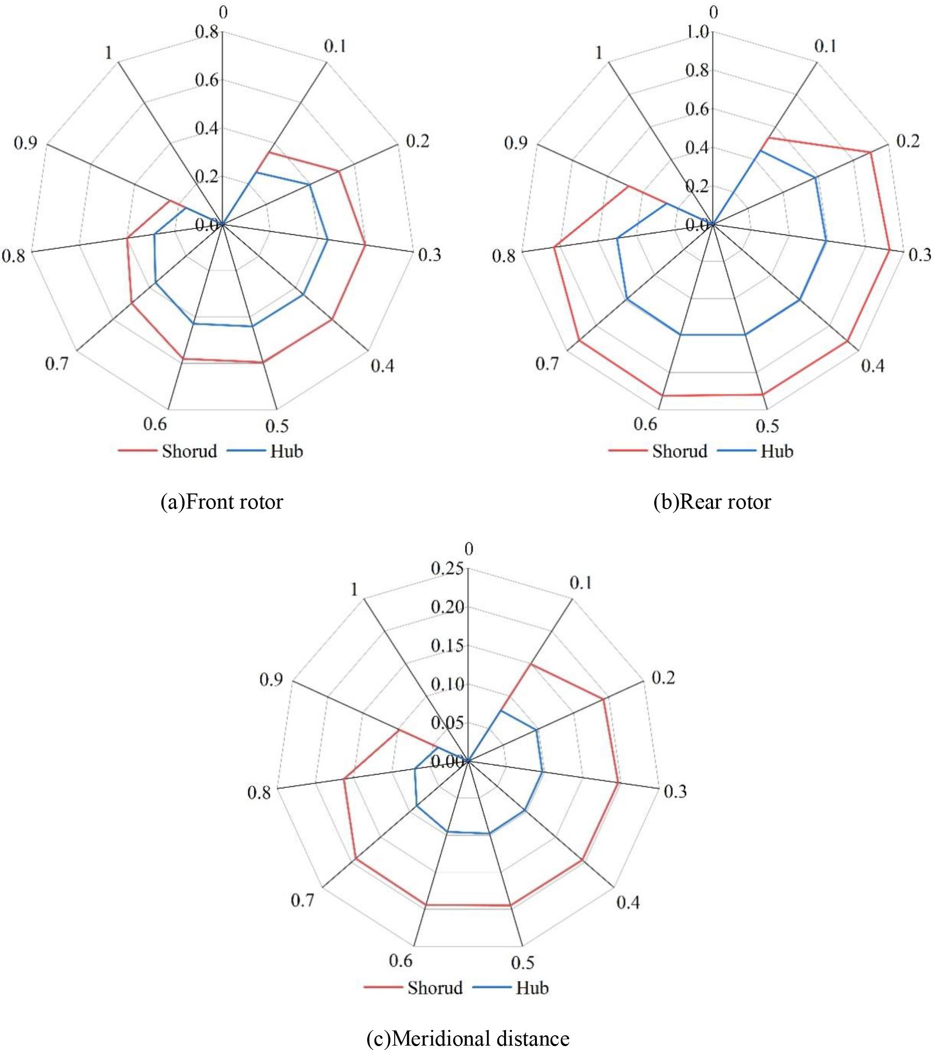
The blade load distribution of the pump propeller
Meanwhile, after obtaining the no-thickness blade, the blade is thickened by using the NACA series of airfoil thickness distribution law to obtain the final pump-jet thruster load distribution design.
After obtaining the geometry of the pump-jet propeller, the pump-jet propeller is placed at the stern of the ship with a finned rudder for numerical self-propelled calculations and analysis of the results under a nonlinear sea state.
The surfaces of the forward and aft rotor blades experience pressure distributions at the design speed, as depicted in Fig. 7. As can be seen from Fig. 7, except for the leading edge where the pressure fluctuation is large due to the violent action of the blade and water (the maximum pressure difference between the pressure distribution on the surface of the front and rear rotor blades is 1199.5 kPa and 1616.8 kPa, respectively), the pressure distribution of the rest of the blade is smooth in the front and rear, and there is no prominent pressure fluctuation, which indicates that the load distribution of the blade is uniform, and there is no region with large pressure gradient, avoiding localised low-pressure areas and reducing cavitation. This indicates that the load distribution of the blade is uniform. There is no region with a large pressure gradient, which avoids the local low-pressure region and reduces the risk of cavitation. This indicates that the load design of the pump-jet thruster under a nonlinear sea state basically meets the design requirements.
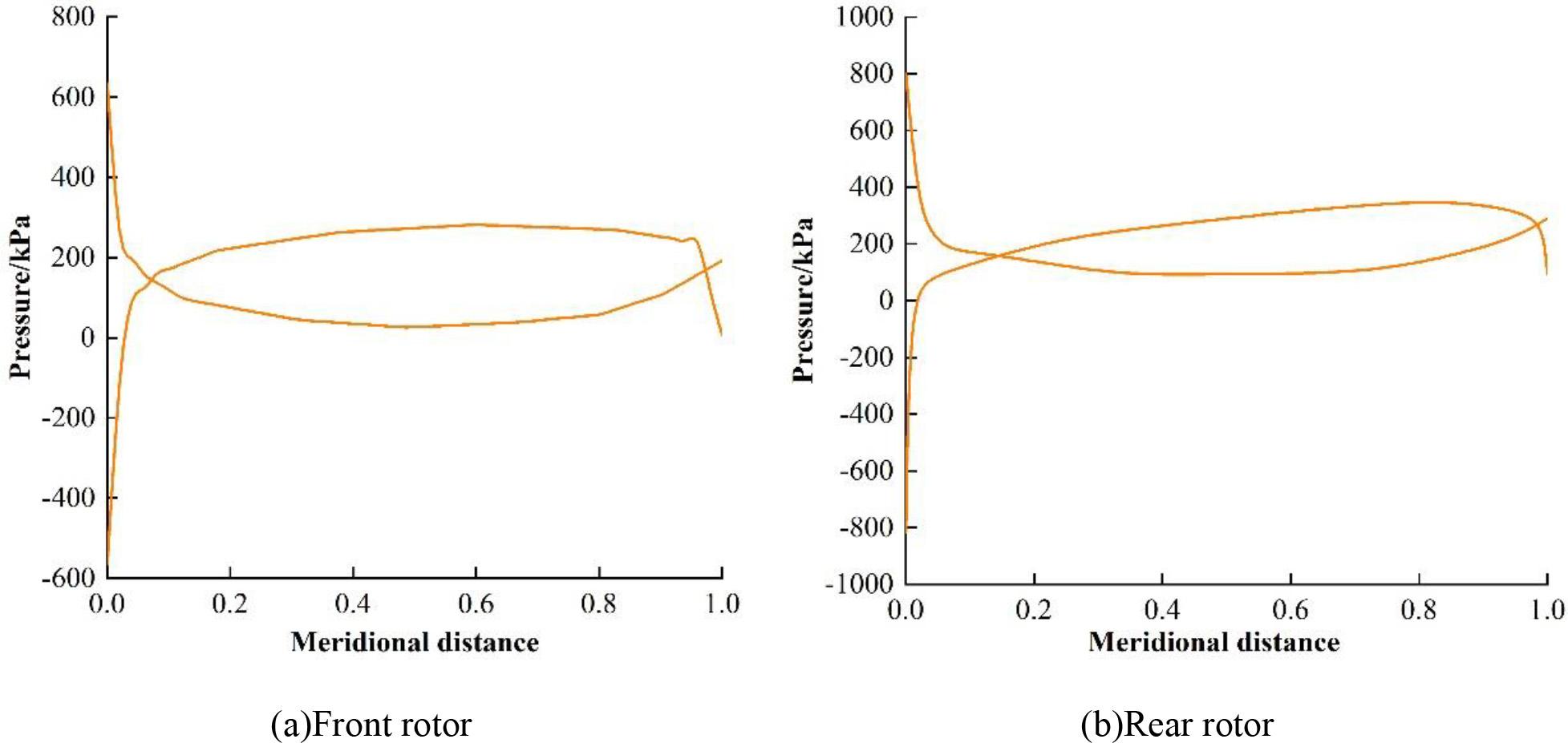
Pressure loading distribution
In this paper, on the basis of nonlinear sea state modelling using second-order Stokes waves and bimodal Ochi-Hubble wave spectra, the CFD-FEM two-way fluid-structure coupling method is used to achieve the prediction and design of the load distribution of the ship’s special mechanical devices and equipments, and the design effect is examined.
This paper takes the pump-jet propeller as the specific research object, and under the wave conditions of wave height H=6m, wavelength to length ratio λ/Lpp=0.87, when the ship sailing against the waves at a speed of 20kn and the waves are thumped, CFD-FEM two-way fluid-solid coupling calculations are carried out for the equidistant measurement points P1~P4 on the pump-jet propeller. The results show that the load at measurement point P4 is seriously affected by the hull thumping, and its peak value exceeds 3.1 kPa. The pressure peaks at measurement points P1 to P4 are flatter and decrease with the height of the measurement point, which is due to the inward tilting of the pump-jet thruster and the negative angle of its inclination rise. The load condition of measurement point P4 obtained by the CFD-FEM two-way fluid-structure coupling method is similar to the experimental results in terms of the hull banging cycle and the amplitude of the load change triggered by the banging action. This indicates the reliability of the CFD-FEM two-way fluid-structure coupling method used in this paper.
Considering the actual sailing conditions of the ship, this paper decides to adopt the intermediate uniform load distribution form that takes into account the efficiency of the pump-jet thruster and cavitation, i.e., the load is maximum at 0.2 chord length and then uniformly distributed and gradually decreases at 0.6 times the chord length. In the load distribution of the designed pump jet thruster, except for the guide edge where the pressure fluctuation is large due to the violent action of the blade and water (the maximum pressure difference between the pressure distribution of the front and rear rotor blade surfaces is 1,199.5kPa and 1,616.8kPa, respectively), the rest of the blade position is smooth in the front and rear pressure distribution, and there is no prominent pressure fluctuation, which indicates that the load distribution of the blade is uniform, and there is no pressure gradient. This indicates that the load distribution of the blade is uniform without a large pressure gradient, which avoids the local low-pressure area and reduces the risk of cavitation. This shows that the load design of the pump-jet thruster under a nonlinear sea state basically meets the design requirements.